A COLLECTION OF FAST ALGORITHMS FOR SCALAR AND VECTOR-VALUED DATA ON IRREGULAR DOMAINS: SPHERICAL HARMONIC ANALYSIS, DIVERGENCE-FREE/CURL-FREE RADIAL BASIS FUNCTIONS, AND IMPLICIT SURFACE RECONSTRUCTION

by
Kathryn Primrose Drake

A dissertation
submitted in partial ful llment
of the requirements for the degree of
Doctor of Philosophy in Computing
Boise State University
December 2020

c 2020
Kathryn Primrose Drake
ALL RIGHTS RESERVED

BOISE STATE UNIVERSITY GRADUATE COLLEGE

DEFENSE COMMITTEE AND FINAL READING APPROVALS

of the dissertation submitted by

Kathryn Primrose Drake

Thesis Title: A Collection of Fast Algorithms for Scalar and Vector-Valued Data on Irregular Domains: Spherical Harmonic Analysis, Divergence Free/Curl-Free Radial Basis Functions, and Implicit Surface Recon struction

Date of Final Oral Examination: 16 October 2020

The following individuals read and discussed the dissertation submitted by student Kathryn Primrose Drake, and they evaluated the students presentation and response to questions during the nal oral examination. They found that the student passed the nal oral examination.

Grady B. Wright Ph.D. Chair, Supervisory Committee
Jodi Mead Ph.D. Member, Supervisory Committee
Min Long Ph.D. Member, Supervisory Committee

The nal reading approval of the dissertation was granted by Grady B. Wright Ph.D., Chair of the Supervisory Committee. The thesis was approved by the Graduate College.

DEDICATION

For Bodie, without whom this wouldnt have been possible.

ACKNOWLEDGMENTS

First and foremost, I must acknowledge and thank my committee members, Professor Jodi Mead and Professor Min Long. Jodi, you have been with me throughout this entire process since (literally) day one. Thank you for supporting me every step of the way and reminding me to persist. Min, you taught me the foundations of scienti computing, and I owe my success in this program in part to you. To my advisor, Grady, this accomplishment feels as much yours as mine. You taught me everything I know, and you saw my potential when I didnt.

I would also like to thank NASA ISGC and the SMART Scholarship, funded by The Under Secretary of Defense-Research and Engineering, National Defense Educa tion Program/BA-1, Basic Research as well as the National Science Foundation grant 1717556. This work was made possible by this nancial support. I must also thank the Mathematics department and Computing program for their continued support. I express my deepest gratitude also to my friends and family, whose constant love and encouragement sustained me. Kayla and Kara, you two are the best of the best. Anna and Shay, I am so fortunate to have siblings who I also consider to be my friends. To my mother, Jennifer, I cannot ever convey how much your words and love mean to me. I am who I am because of you.

Finally, my husband, Bodie. You are the best partner, companion, and friend. Thank you for choosing this life and chasing this dream with me. We did it!

ABSTRACT

This dissertation addresses problems that arise in a diverse group of elds includ ing cosmology, electromagnetism, and graphic design. While these topics may seem disparate, they share a commonality in their need for fast and accurate algorithms which can handle large datasets collected on irregular domains. An important issue in cosmology is the calculation of the angular power spectrum of the cosmic microwave background (CMB) radiation. CMB photons o er a direct insight into the early stages of the universes development and give the strongest evidence for the Big Bang theory to date.

The Hierarchical Equal Area isoLatitude Pixelation (HEALPix) grid is used by cosmologists to collect CMB data and store it as points on the sphere. HEALPix also refers to the software package that analyzes CMB maps and calculates their an gular power spectrums. Re ned analysis of the CMB angular power spectrum can lead to revolutionary developments in understanding the curvature of the universe, dark matter density, and the nature of dark energy. In the rst paper, we present a new method for performing spherical harmonic analysis for HEALPix data, which is a vital component for computing the CMB angular power spectrum.

Using numerical experiments, we demonstrate that the new method provides better accuracy and a higher convergence rate when compared to the current methods on synthetic data. This paper is presented in Chapter 2. The problem of constructing smooth approximants to divergence-free (div-free)

and curl-free vector elds and/or their potentials based only on discrete samples arises in science applications like uid dynamics and electromagnetism. It is often necessary that the vector approximants preserve the div-free or curl-free properties of the eld. Div/curl-free radial basis functions (RBFs) have traditionally been uti lized for constructing these vector approximants, but their global nature can make them computationally expensive and impractical. In the second paper, we develop a technique for bypassing this issue that combines div/curl-free RBFs in a partition of unity (PUM) framework, where one solves for local approximants over subsets of the global samples and then blends them together to form a div-free or curl-free global approximant.

This method can be used to approximate vector elds and their scalar potentials on the sphere and in irregular domains in R2 and R3. We present error estimates and demonstrate the e ectiveness of the method on several test problems. This paper is presented in Chapter 3.

The issue of reconstructing implicit surfaces from oriented point clouds has appli cations in computer aided design, medical imaging, and remote sensing. Utilizing the technique from the second paper, we introduce a novel approach to this problem by exploiting a fundamental result from vector calculus. In our method, deemed CFPU, we interpolate the normal vectors of the point cloud with a curl-free RBF-PUM inter polant and extract a potential of the reconstructed vector eld. The zero-level surface of this potential approximates the implicit surface of the point cloud. Bene ts of this method include its ability to represent local sharp features, handle noise in the normal vectors, and even exactly interpolate a point cloud. We demonstrate in the third paper that our method converges for known surfaces and also show how it performs on various surfaces found in the literature. This paper is presented in Chapter 4.

LIST OF FIGURES

1.1 A C M B temperature anisotropy map [28]. . . . . . . . . . . . . . . .

1.2 A portion of the C M B as measured by (a) C O B E in 1992 [30], (b) W M A Pin 2003 [3], and (c) Planck in 2013 [28]. . . . . . . . . . . . .

1.3 Illustration of a region of higher density falling into a gravitational potential well using the system of a mass on a spring [15]. . . . . . .

1.4 Peaks in the angular power spectrum of C M B temperature anisotropies T and how they correspond to the compression and rarefaction of the baryon-photon uid in the early universe [15]. . . . . . . . . . . . . .

1.5 A reconstruction of a drainage surface using RBF interpolation on scattered points. . . . . . . . . . . . . . . . . . . . . . . . . . . . . . .

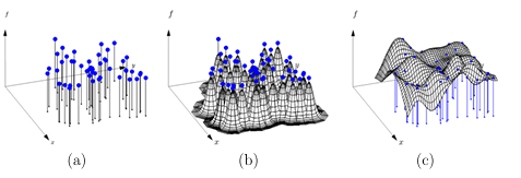
1.6 The process of using R B F s to interpolate a set of scattered data in 2 D: (a) a target function f sampled at some set of distinct nodes, (b) a set of radial basis functions interpolating the data, and (c) a reconstructed surface resulting from the interpolation . . . . . . . . . . . . . . . . .

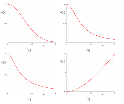
1.7 (a)The Gaussian ( = 2), (b) inverse quadric ( = 3.5), (c) inverse multiquadric ( = 6), and (d) multiquadric radial kernels ( = 2) from Table 1.1. . . . . . . . . . . . . . . . . . . . . . . . . . . . . . . . . .

2.1 C M B component map from the Planck mission [30] (a) and correspond ing (scaled) angular power spectrum (b). . . . . . . . . . . . . . . . .

2.2 HEALPix grid with resolutions, from left to right, Nside = 1248. The lines indicate the pixel boundaries and the solid dots represent the pixel centers or points. . . . . . . . . . . . . . . . . . . . . . . . .

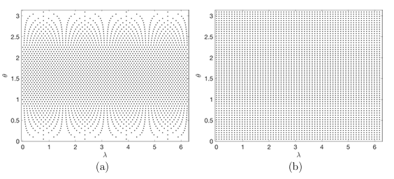
2.3 H E A L Pix grid on [02 ] [0 ], where islatitude, and is longitude. The point sets in the northern (N), equatorial (E), and southern (S) regions are shown in blue, red, and yellow, respectively. . . . . . . . .

2.4 (a) HEALPix points with Nside = 16 displayed in latitude and longitude and (b) the corresponding upsampled points. . . . . . . . . . . .

2.5 Illustration of the DFS method: (a) The surface of earth, (b) the surface mapped onto a latitude-longitude grid, and (c) the surface after applying the D F S method. [40] . . . . . . . . . . . . . . . . . . . . .

2.6 Maximum absolute errors as a function of t for the computed spherical harmonic coefficients of (2.20) using HP 2 S PH and (a) H E A L Pix (3 it erative refinement steps), pixel weights, ring weights and (b) H EA L Pix with increasing iterative steps. The lines in the figure are the lines of best t to the data and the convergence rates are determined from the slope of this line (as displayed in the plot legends). . . . . . . . . . .

2.7 Maximum absolute errors as a function of t for the computed spherical harmonic coefficients of (2.20) augmented with spherical harmonics using H P 2 S P H,HEAL Pix with 3 iterative refinement steps, pixel weights, and ring weights. . . . . . . . . . . . . . . . . . . . . . . . . . . . . .

2.8 (a) Scaled angular power spectrum of (2.20) as a function of degree computed by the HEALPix software with 3 iterative re nement steps, the HP2SPH method, the HEALPix method with ring weights, and the HEALPix method with pixel weights. The exact power spectrum is given by the black s. Here Nside = 210, which is N = 12 582 912
total points. (b) Absolute errors in the (scaled) angular power spec trum of the results from (a) as a function of degree . . . . . . . . . .
2.9 Absolute errors in the (scaled) angular power spectrum of (2.20) aug- mented with high-degree spherical harmonics computed by the HEALPix software with 3 iterative re nement steps, the HP2SPH method, the HEALPix method with ring weights, and the HEALPix method with pixel weights as a function of degree . (a) Displays the errors for degrees 450 = 1 2000, while (b) displays the errors only for = 1500 to better show the how good the methods are at recover ing the spectrum at the degrees of the appended spherical harmonics. Here Nside = 210, which is N = 12 582 912 total points. . . . . . . .

2.10 (Scaled) angular power spectrum of the CMB data map displayed in Figure 2.1 (a) with Nside = 211 for the four methods discussed in the paper (left), and the relative errors of the HEALPix software methods against the HP2SPH method (right). . . . . . . . . . . . . . . . . . .

3.1 (a) Illustration of partition of unity patches (outlined in blue lines) for a node set X (marked with black disks) contained in a domain (marked with a dashed line). (b) Illustration of one of the PU weight functions for the patches from part (a), where the color transition from white to yellow to red to black correspond to weight function values from 0 to 1. . . . . . . . . . . . . . . . . . . . . . . . . . . . . . . . .

3.2 Div-free R BF partition of unity approximant of the potential from Section 3.5.1 (a) without the patch potentials shifted ( k) (b) with the patch potentials shifted ( k). . . . . . . . . . . . . . . . . . . . . . .

3.3 Illustration of the glue points for shifting the potentials. The asterisks denote the glue points and the small circles denote the patch centers.

3.4 Contours of the potential (1) (left) and corresponding div-free velocity eld u(1) div (right) for the numerical experiment on R2. . . . . . . . . .

3.5 Convergence results for the numerical experiment on the star domain in R2 for the IMQ kernel and di erent values of q. Filled (open) markers correspond to the relative-norm (2-norm) errors and solid (dashed) lines indicate the t to the estimate E(N) = e Clog(N)N1 4, without the rst values included. . . . . . . . . . . . . . . . . . . . . . . . . . .

3.6 Contours of the potential (2) (left) and corresponding div-free velocity eld u(2) div(right) for the numerical experiment on S2. . . . . . . . . . .

3.7 Convergence rates for the numerical experiment on S2 for the Matern kernel and di erent values of q. Filled (open) markers correspond to the relative-norm (2-norm) errors and solid (dashed) lines indicate the lines of best t to the-norm (2-norm) errors as a function of N on a loglog scale. The legend indicates the slopes of these lines
with the rst number corresponding to the-norm and the second the 2-norm, which give estimates for the algebraic convergence rates.

3.8 Timing results for the numerical experiment on S2 with di erent values of q. The dashed lines are the lines of best t to the timings using all but the rst two values. . . . . . . . . . . . . . . . . . . . . . . . . .

3.9 (a) Visualization of the potential (3) and corresponding curl-free ve locity eld u(3) curl = (3) for the numerical experiment on the unit ball. (b) Example of N = 4999 node set (small solid disks) used in the numerical experiment on the unit ball, where colors of the nodes are proportional to their distance from the origin (yellow=1, green = 0.5, blue=0). The plots in both gures show the unit ball with a wedge removed to aid in the visualization. . . . . . . . . . . . . . . . . . . .

3.10 Convergence results for the numerical experiment on the unit ball in R3 for the IMQ kernel and di erent values of q. Filled (open) markers cor respond to the relative-norm (2-norm) errors and solid (dashed) lines indicate the t to the expected error estimate E(N) = e Clog(N)N1 6, without the rst values included. . . . . . . . . . . . . . . . . . . . .

4.1 (a) N = 30 points sampled from a Cassini oval (4.11) with a = 1 and b = 11, together with the corresponding normal vectors to the curve. (b) The reconstruction from the global curl-free PHS interpolation method (magenta) with the exact curve (blue dashed line). . . .

4.2 (a) N =6144 point cloud and corresponding normals for the knot. (b) CFPU reconstruction of the knot from the data in part (a). . . . . . .

4.3 Comparison of the CFPU reconstructions of the knot with zero mean Gaussian white noise added to the normals. First column shows the reconstructions without any regularization. Second and third columns show the reconstructions using regularization with a xed parameter chosen for all the patches. Fourth column shows the reconstructions with the regularization parameter chosen using GCV on each patch. All results use N = 23064 samples and M = 864 patches with a xed patch radius of = 3 4. . . . . . . . . . . . . . . . . . . . . . . . . .

4.4 CFPU reconstructions of the Stanford bunny with (a) no regularization and (b) with regularization. In (b) GCV was used to determine the regularization parameter on each patch. Both experiments used the highest resolution zippered model of the bunny consisting of N = 35947 points and normals vectors and M = 848 patches. . . . . . . . . . . .

4.5 C F P U reconstructions of the Stanford bunny with (a) no regularization and (b) with regularization. In (b) GCV was used to determine the regularization parameter on each patch. Both experiments used the highest resolution zippered model of the bunny consisting of N = 35947 points and normals vectors and M = 848 patches. . . . . . . . . . . .

4.6 CFPUreconstructions of the Dragon with (a) no regularization and (b) with regularization. In (b) GCV was used to determine the regular ization parameter on each patch. Both experiments used the highest resolution zippered model of the dragon consisting of N = 436418 points and normals vectors and M = 14400 patches. . . . . . . . . . .

4.7 CFPU reconstructions of the Armadillo with (a) no regularization and (b) with regularization. In (b) GCV was used to determine the regularization parameter on each patch. Both experiments used the highest resolution zippered model of the dragon consisting of N = 172974 points and normals vectors and M = 14349 patches. . . . . . . . . . .

4.8 CFPUreconstructions of the Happy Buddha with (a) no regularization and (b) with regularization. In (b) GCV was used to determine the regularization parameter on each patch. Both experiments used the highest resolution zippered model of the dragon consisting of N = 583079 points and normals vectors and M = 14226 patches. . . . . .

LIST OF TABLES

1.1 Commonly used radial kernels, where the rst three are positive de nite, r = x y , and is the shape parameter. . . . . . . . . . . . .

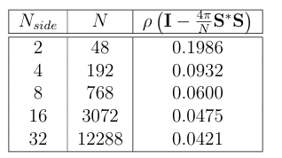
2.1 Spectral radius of the Richardson iteration matrix from (2.6) for dif ferent values of N. . . . . . . . . . . . . . . . . . . . . . . . . . . . .

4.1 Examples of radial kernels that result in positive de nite matrices A (4.5) for curl-free RBF interpolation. Here > 0 is the shape parameter.

4.2 Comparison of the errors in the CFPU reconstruction of the knot for increasing numbers of samples N using the curl-free PHS kernel , for =12. All results use a xed number of M = 864 PU patches and axed patch radius of = 3 4. . . . . . . . . . . . . . . . . . . . . . .

CHAPTER 1:
INTRODUCTION

This dissertation develops a collection of fast and accurate algorithms for anal yzing large datasets collected on the sphere as well as other irregular domains. It is composed of three papers. The rst paper [9] is inspired by the Cosmic Microwave Background (CMB) radiation and describes a new technique for spherical harmonic analysis of data collected on the HEALPix grid. The second paper [7] introduces a method for approximating divergence-free and curl-free vector elds on irregular domains in R2, the sphere, and R3 using radial basis functions and the partition of unity method. The third paper [8] utilizes the technique from [7] for curl-free elds in a novel approach for surface reconstruction from oriented point cloud data. In this introduction, I provide a motivation for each of these papers as well as relevant background information.

1.1 Cosmic Microwave Background Radiation
Angular Power Spectrum

The Cosmic Microwave Background (CMB) radiation represents the rst light to travel during the early stages of the universes development and gives the strongest evidence for the Big Bang theory to date. Re ned analysis of the CMB angular power spectrum can lead to revolutionary developments in understanding the nature of dark matter and dark energy. CMB data is collected on the Hierarchical Equal Area isoLatitude Pixelation (HEALPix) grid, which has associated software for calculating its angular power spectrum. In this section, we o er pertinent motivational and background information to our paper, which is given in Chapter 2.

1.1.1 Motivation

Light from the CMB is nearly as old as the universe itself. This relic radiation allows us to look into the past and see the universe as it was in its infancy, only 379,000 years after the Big Bang. In fact, the existence of the CMB provides the strongest evidence for the theory of the Big Bang [3]. According to the Big Bang theory, the universe began as a dense plasma of matter, too hot for even light to travel. As the universe expanded, however, this particle soup gradually cooled until nally the temperature dropped below 3000K. This is the temperature threshold at which atomic hydrogen formed for the rst time (deemed the Epoch of Recombination), allowing photons to travel freely. These photons make up the CMB we see today and appear to come from a spherical surface all around us, now averaging a temperature of 27K. While the CMB has been deemed the most perfect black body ever measured in nature [37], there are minute temperature di erences on the level of 1 part in 100000. Usually the CMB is presented as a sphere composed of various colors which represent these
temperature anisotropies, as shown in Figure 1.1.

When the CMB was discovered in 1965, it was detected accidentally using a radio telescope [27]. Since then, ground-based telescopes, balloons, and satellites have all been used to measure the CMB temperature uctuations at increasingly small angular scales of the sky (Figure 1.2). These temperature anisotropies are important because they are actually imprints of conditions in the early universe. It is theorized that the

Figure 1.1 A CMB temperature anisotropy map [28].

tiny density uctuations in the primordial plasma grew into the large-scale structures of stars, galaxies, and even clusters of galaxies that we see today. Cosmologists can ascertain the curvature as well as the content of matter and energy in the universe using the angular power spectrum of CMB temperature maps [3, 14].

Figure 1.2 A portion of the CMB as measured by (a) COBE in 1992 [30],(b) WMAP in 2003 [3], and (c) Planck in 2013 [28].

1.1.2 Background

Once a CMB temperature map is composed, it can then be analyzed by its angular power spectrum (Figure 1.4). This power spectrum can be viewed as a measurement of the temperature uctuations against an angular wavenumber, more commonly referred to as the multipole . The multipole is related to the inverse of the angular scale of the sky and is derived from a spherical harmonic decomposition of the sky. Spherical harmonic coe cients amof the CMB map are used to calculate the angular power spectrum:

1.1
The peaks of the CMB temperature power spectrum at higher multipoles (i.e. smaller angular scales) are what hold the key to the infant universe. Before the Epoch of Recombination, the majority of the matter in the universe was a plasma of electrons, protons, and CMB photons. We refer to this as the photon baryon plasma or uid, where baryon is a general term for ordinary matter that has mass. Quantum uctuations in the early universe created gravitational potential wells, which attracted the matter around them. As matter collected in these wells the photon-baryon uid was compressed, increasing the pressure and temperature of the plasma. This pressure built until the compression was reversed, creating an oscillating sequence of compression and rarefaction. One can visualize this process as a mass on a spring falling under gravity, where the radiation pressure is the spring,
and the energy density of the uid is the mass (see Figure 1.3). Note that dark matter only interacts with gravity, not light or pressure, so only the photon-baryon plasma was oscillating. Analogous to traveling compressional waves in the air being perceived as sound, these oscillations in the photon-baryon uid are called acoustic oscillations. At the time of recombination, the photon-baryon uid stopped oscillating, making it so that the pattern of the sound waves are imprinted on the temperature of the

Figure 1.3 Illustration of a region of higher density falling into a gravita-tional potential well using the system of a mass on a spring [15].

CMB. Extrema in the oscillations become the peaks in the CMB power spectrum, where odd peaks correspond to plasma compression and the even peaks correspond to plasma rarefaction, as shown in Figure 1.4. Because of this connection, the tempera ture power spectrum is sensitive to fundamental cosmological parameters, speci cally in regard to the density of dark matter in the universe. Cosmologists can make theoretical calculations of the CMB power spectrum based on the values of these pa rameters and compare it to the observed angular power spectrum [37]. The location of the rst peak provides insight to the curvature of the universe, the amplitude of the second peak will tell us about the baryon density, and the amplitude of the third peak will tell us about the density of dark matter [16]. Note from Figure 1.4 that these peaks occur at high .

The challenge to computing the CMB angular power spectrum is to use a method for calculating the spherical harmonic coe cients from the CMB data that is as accurate as possible. It is especially important for the technique used to be sensitive to data at high multipoles. Our paper [9] address precisely this issue by introducing a novel method for calculating the CMB angular power spectrum which demonstrates better accuracy across all multipoles on test data.

Figure 1.4 Peaks in the angular power spectrum of CMB temperature anisotropies T and how they correspond to the compression and rarefaction of the baryon-photon uid in the early universe [15].

1.2 Scalar Radial Basis Function Interpolation

A common problem that arises in many disciplines is that of approximating vector elds, or scalar potentials for the elds, based only on scattered samples. The method developed in [7] is the rst to implement divergence-free (div-free) and curl-free vector valued RBF approximation with a partition of unity. An added bene t of the method
is that it produces an approximant for the scalar potential of the underlying sampled eld as well. This section o ers pertinent motivational and background information to our paper, which is given in Chapter 3.

1.2.1 Motivation

Approximating vector fields from scattered samples is a problem that arises in many scientific applications, including, for example, uid dynamics, meteorology, magneto hydrodynamics, electro magnetics, gravitational lensing, imaging, and computer graphics. These vector elds often have the additional property of being either div free or curl-free. For example, div-free vector elds represent incompressible uid flows and (static) magnetic elds, while curl-free vector elds represent gravity elds and (static) electric elds. When developing a method for approximating vectors fields, it is important to ensure that the approximant preserves the div-free/curl-free nature of the eld or problems can arise. For instance, in incompressible ow simu lations using the immersed boundary method, excessive volume loss can occur if the approximated velocity eld of the uid is not div-free [2]. To enforce these di erential invariants on the approximant, one can not approximate the individual components of the eld separately, but must combine them in a particular way. Div/curl-free radial basis functions (RBFs) are a particularly good choice for this application as they are meshfree and the vector approximants analytically satisfy the div-free or curl-free property. A negative aspect of this approach, however, is that the method is computationally expensive due to its global nature. One of the ways to overcome this issue is to combine vector RBF approximation with a local technique like the partition of unity method.

1.2.2 Background

Interpolating scattered data is a problem that emerges in multiple scienti c disciplines and applications, such as meteorology, electronic imaging, computer graphics, medicine, and the Earth sciences [11, 1, 19, 31, 25]. RBF interpolation was introduced by R.L. Hardy in 1968 to solve a common problem in cartography of nding a contin uous function that accurately represents a surface given sparse measurements [12, 13] (see Figure 1.5 for an example). Geometrically, the RBF method can be viewed as

Figure 1.5 A reconstruction of a drainage surface using RBF interpolation on scattered points.

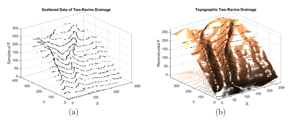
interpolating data with a linear combination of translates of a single basis function, (r), that is radially symmetric about its center. This process can be seen graphically in Figure 1.6. Mathematically, the interpolation process is de ned as follows. Given

Figure 1.6 The process of using RBFs to interpolate a set of scattered data in 2D: (a) a target function f sampled at some set of distinct nodes, (b) a set of radial basis functions interpolating the data, and (c) a reconstructed surface resulting from the interpolation

adistinct setof scatterednodesY= yj }N j=1 Rd and some scalar-value dtarget function fsampledatY,thescalar-valued RBF interpolantof fY isgivenby

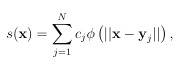
1.2

wherex Rd, isthed-dimensionalEuclideannorm,and (r)issomeradialkernel. The expansioncoe cients cj can be determined by solving the symmetric linear system formed by enforcing the interpolation condition s s (yj)=fj j=1 N:

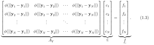
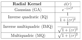
Several options for the radial kernel (r)have been developed that ensure the inter polation matrix AY will be unconditionally non singular, i.e., that the linear system in(1.3)will be uniquely solvable [22]. Table 1.1 lists some of the most commonly use dones of these radial kernels,and Figure 1.7 shows plots of theskernels. Sinceits introduction,R B F interpolation has be com increasingly popular in applications such as computer animation,medical imaging,and fluid dynamics. Unfortunately,due to its global nature,the computational cost of solving for the interpolation coefficient scan be prohibitive for large N. One of the techniques that has been
used to overcome this issue is the partition of unity method(P UM). In R BF-P UM, one only need s to solve fo r local approximants over small subsets of the global dataset

Table 1.1 Commonly used radial kernels, where the rst three are positive de nite, r = x y , and is the shape parameter.

Figure 1.7 (a)The Gaussian ( = 2), (b) inverse quadric ( = 35), (c) inverse multiquadric ( = 6), and (d) multiquadric radial kernels ( = 2) from Table
1.1

and then blend them together to form a smooth global approximant [18, 35, 10, 6, 17]. In general,a partition of unity is defined as a collection of weight functions w M =1

subordinate to the open cover of a domain , i.e.Ml=1 , such that

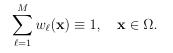
A global interpolant s to f over the whole domain is calculated by blending local RBF interpolants s of the form (1.2) with the partition of unity weight functions:

1.4

The localized approach of RBF-PUM allows for all of the bene ts of RBF interpolation without the drawback of computational bottleneck. While this method works well for interpolating scalar-valued functions, it has not been extended for div-free/curl free vector elds. Our paper [7] introduces the rst vector-valued RBF-PUM for approximating div-free and curl-free vector fields.

1.3 Implicit Surface Reconstruction from Oriented Point Clouds

The nal topic addressed in this dissertation is that of surface reconstruction from a set of unorganized points. This process has applications in a variety of domains, including computer graphics, computer-aided design, medical imaging, image pro cessing, and manufacturing. Many common methods developed to address this problem require Hermite data or oriented point clouds, which involve the unstructured points as well as their corresponding normal vectors. In [8] we present a novel method for reconstructing surfaces from Hermite data titled Curl-free Radial Basis Function Partition of Unity (CFPU). This section o ers background information to our paper,

which is given in Chapter 4.

1.3.1 Motivation

A point cloud is a set of unorganized points, usually in 3D space. Often a collection of points is produced by a scanner measuring an object or surface. Analyzing, processing, and characterizing point clouds arises in the areas of computer vision, medical imaging, and engineering. It is desirable to have an implicit surface representation of point clouds because it allows for a mathematical description which can then be rendered at any resolution as well as allow for informative calculus operations to be performed. Additionally, while point clouds are not watertight, regular implicit surface are watertight, which is vital in many applications.

Reconstructing implicit surfaces from oriented point clouds has been extensively studied in literature since the 90s, with many approaches based on RBFs [23, 24, 26, 29, 32, 34, 20, 21, 4, 33, 36, 5]. Due to the global nature of RBF methods, they suer from an inability to reconstruct ner details of a surface as well as being too slow for larger point cloud datasets. To bypass this issue, we combine curl-free RBF approximation with the partition of unity method. This allows for recovery of a global zero-level implicit surface to the point cloud from computations performed on local patches. An added bene t of this approach is that it is better equipped to recover sharp features, which many global methods lack. Additionally, the method can be adapted to enforce exact interpolation of the surface and can be regularized to handle noisy data. Finally, we develop a version of the method that is free of shape or scaling parameters, which are common to other RBF methods and for which good values are computationally expensive to determine automatically. The method presented in this paper is an extension of the algorithm in paper 2, and as such, all of the pertinent background information is covered in Section 2.

1.4 Overview of the Dissertation

The remainder of the dissertation is as follows. Author contributions for papers 1, 2, and 3 are provided in chapters 2, 3, and 4, respectively. Chapter 5 o ers concluding remarks and future directions for research on the topics of the dissertation. The appendices contain the papers that make up the bulk of the discoveries and advances of the thesis.

REFERENCES

[1] I. Amidror. Scattered data interpolation methods for electronic imaging systems: a survey. J. Electron. Imaging., 11:157176, 2002.
[2] Y. Bao, A. Donev, B. E. Gri th, D. M. McQueen, andC.S.Peskin. An immersed boundary method with divergence-free velocity interpolation and force spreading. J. Comput. Phys., 347:183206, 2017.
[3] C. L. Bennett, D. Larson, J. L. Weiland, N. Jarosik, G. Hinshaw, N. Odegard, K. M. Smith, R. S. Hill, B. Gold, M. Halpern, E. Komatsu, M. R. Nolta, L. Page,
D. N. Spergel, E. Wollack, J. Dunkley, A. Kogut, M. Limon, S. S. Meyer, G. S. Tucker, and E. L. Wright. Nine-year wilkinson microwave anisotropy probe (WMAP) observations: Final maps and results. The Astrophysical Journal Sup plement Series, 208(2):20, 2013.
[4] J. C. Carr, R. K. Beatson, J. B. Cherrie, T. J. Mitchell, W. R. Fright, B. C. McCallum, and T. R. Evans. Reconstruction and representation of 3d objects with radial basis functions. In Proceedings of the 28th Annual Conference on Computer Graphics and Interactive Techniques, pages 6776, 2001.
[5] J. C. Carr, W. R. Fright, and R. K. Beatson. Surface interpolation with radial basis functions for medical imaging. IEEE Transactions on Medical Imaging, 16(1):96107, 1997.

[6] R. Cavoretto and A. De Rossi. Fast and accurate interpolation of large scattered data sets on the sphere. Comput. Appl. Math., pages 15051521, 2010.
[7] K. P. Drake, E. J. Fuselier, and G. B. Wright. A divergence-free and curl-free radial basis function partition of unity method. arXiv:2010.15898, 2020.
[8] K. P. Drake, E. J. Fuselier, and G. B. Wright. Implicit surface reconstruction with a curl-free radial basis function partition of unity method. To be submitted, 2020.
[9] K. P. Drake and G. B. Wright. A fast and accurate algorithm for spherical harmonic analysis on HEALPix grids with applications to the cosmic microwave background radiation. Journal of Computational Physics, 416:109544, 2020.
[10] G. E. Fasshauer. Meshfree Approximation Methods with MATLAB, Interdisci plinary Mathematical Sciences. World Scienti c Publishers, Singapore, 2007.
[11] R. Franke. Approximation of Scattered Data for Meteorological Applications. Birkhauser Basel, Basel, 1990.
[12] R. L. Hardy. Multiquadric equations of topography and other irregular surfaces. J. Geophy. Res., 76:19051915, 1971.
[13] R. L. Hardy. Theory and applications of the multiquadric-biharmonic method: 20 years of discovery. Comput. Math. Appl., 19:163208, 1990.
[14] G. Hinshaw, D. Larson, E. Komatsu, D. N. Spergel, C. L. Bennett, J. Dunkley, M. R. Nolta, M. Halpern, R. S. Hill, N. Odegard, L. Page, K. M. Smith, J. L. Weiland, B. Gold, N. Jarosik, A. Kogut, M. Limon, S. S. Meyer, G. S. Tucker,

E. Wollack, and E. L. Wright. Nine-year wilkinson microwave anisotropy probe (WMAP) observations: cosmological results. The Astrophysical Journal Supple ment Series, 208(2):19, 2013.
[15] W. Hu. ate guide Ringing to the in acoustic the new cosmology: peaks and Intermedi polarization,
http://background.uchicago.edu/ whu/intermediate/intermediate.html. 2001.
[16] W. Hu. CMB temperature and polarization anisotropy fundamentals. Annals of Physics, 303(1):203225, 2003.
[17] E. Larsson, V. Shcherbakov, and A. Heryudono. A least squares radial basis function partition of unity method for solving PDEs. SIAM J. Sci. Comput., 39(6):A2538A2563, 2017.
[18] D. Lazzaro and L. B. Montefusco. Radial basis functions for the multivariate interpolation of large scattered data sets. J. Comp. Appl. Math., 140(1):521536, 2002.
[19] J. P. Lewis, F. Pighin, and K. Anjyo. Scattered data interpolation and approxi mation for computer graphics. In ACM SIGGRAPH ASIA 2010 Courses, page 2. ACM, 2010.
[20] S. Liu, C. C. Wang, G. Brunnett, and J. Wang. A closed-form formulation of
HRBF-based surface reconstruction by approximate solution. Comput. Aided Des., 78(C):147157, 2016.
[21] I. Macedo, J. P. Gois, and L. Velho. Hermite radial basis functions implicits. Computer Graphics Forum, 30(1):2742, 2011.

[22] C. A. Micchelli. Interpolation of scattered data: distance matrices and conditionally positive de nite functions. Constr. Approx., 2:1112, 1986.
[23] B. S. Morse, T. S. Yoo, P. Rheingans, D. T. Chen, and K. R. Subramanian. Interpolating implicit surfaces from scattered surface data using compactly sup ported radial basis functions. In Proceedings International Conference on Shape Modeling and Applications, pages 8998, 2001.
[24] Y. Ohtake, A. Belyaev, and H. P. Seidel. 3D scattered data interpolation and ap proximation with multilevel compactly supported RBFs. Graph Models, 67:150 165, 2005.
[25] E. Oubel, M. Koob, C. Studholme, J. L. Dietemann, and F. Rousseau. Recon struction of scattered data in fetal di usion mri. Medical Image Computing and Computer-Assisted InterventionMICCAI 2010, pages 574581, 2010.
[26] R. Pan, X. Meng, and T. Whangbo. Hermite variational implicit surface recon struction. Sci China Ser F, 52(2):308315, 2009.
[27] A. A. Penzias and R. W. Wilson. A measurement of excess antenna temperature at 4080 mc/s. The Astrophysical Journal, 142:419421, 1965.
[28] Planck Collaboration 2005. Planck: The scienti c programme. ESA publication ESA-SCI(2005)/01, 2005.
[29] M. Samozino, M. Alexa, P. Alliez, and M. Yvinec. Reconstruction with voronoi centered radial basis functions. In Proceedings of the fourth Eurographics sym posium on geometry processing, pages 5160, 2006

[30] G. F. Smoot, C. L. Bennett, A. Kogut, E. L. Wright, J. Aymon, N. W. Boggess, E. S. Cheng, G. de Amici, S. Gulkis, M. G. Hauser, G. Hinshaw, P. D. Jackson, M. Janssen, E. Kaita, T. Kelsall, P. Keegstra, C. Lineweaver, K. Loewenstein,
P. Lubin, J. Mather, S. S. Meyer, S. H. Moseley, T. Murdock, L. Rokke, R. F. Silverberg, L. Tenorio, R. Weiss, and D. T. Wilkinson. Structure in the COBE di erential microwave radiometer rst-year maps. The Astrophysical Journal, 396:L1L5, 1992.
[31] G. J. Streletz, G. Gebbie, O. Kreylos, B. Hamann, L. H. Kellogg, and H. J. Spero. Interpolating sparse scattered data using ow information. Journal of Computational Science, 16:156169, 2016.
[32] J. Sussmuth, Q. Meyer, and G. Greiner. Surface reconstruction based on hier archical oating radial basis functions. Comput Graph Forum, 29(6):1854 1864, 2010.
[33] G. Turk and J. F. OBrien. Modeling with implicit surfaces that interpolate. ACM Trans Graph, 21(4):855873, 2002.
[34] C. Walder, B. Scholkopf, and O. Chapelle. Implicit surface modeling with a globally regularised basis of compact support. Comput Graph Forum, 25(3):635 644, 2006.
[35] H. Wendland. Fast evaluation of radial basis functions : Methods based on partition of unity. In Approximation Theory X: Wavelets, Splines, and Applications, pages 473483. Vanderbilt University Press, 2002.

[36] H. Wendland. Scattered Data Approximation, volume 17 of Cambridge Monogr. Appl. Comput. Math. Cambridge University Press, Cambridge, 2005.
[37] M. White. Anisotropies in the CMB. Proceedings of Division of Particles and Fields of the American Physical Society, 1999.

CHAPTER 2:

A FAST AND ACCURATE ALGORITHM FOR SPHERICAL HARMONIC ANALYSIS ON HEALPIX GRIDS WITH APPLICATIONS TO THE COSMIC MICROWAVE BACKGROUND RADIATION

Kathryn P. Drake1 and Grady B. Wright
Journal of Computational Physics, 416:109544, 2020.

Abstract

The Hierarchical Equal Area isoLatitude Pixelation (HEALPix) scheme is used extensively in astrophysics for data collection and analysis on the sphere. The scheme was originally designed for studying the Cosmic Microwave Background (CMB) radiation, which represents the rst light to travel during the early stages of the universes development and gives the strongest evidence for the Big Bang theory to date. Re ned analysis of the CMB angular power spectrum can lead to revolutionary developments in understanding the nature of dark mat 1Corresponding author.

ter and dark energy. In this paper, we present a new method for performing spherical harmonic analysis for HEALPix data, which is a central component to computing and analyzing the angular power spectrum of the massive CMB data sets. The method uses a novel combination of a non-uniform fast Fourier transform, the double Fourier sphere method, and Slevinskys fast spherical harmonic transform [38]. For a HEALPix grid with N pixels (points), the com putational complexity of the method is O(N log2 N), with an initial set-up cost of O(N3 2logN). This compares favorably with O(N3 2) runtime complexity of the current methods available in the HEALPix software when multiple maps need to be analyzed at the same time. Using numerical experiments, we demon strate that the new method also appears to provide better accuracy over the entire angular power spectrum of synthetic data when compared to the current methods, with a convergence rate at least two times higher.

2.1 Introduction

About 379,000 years after the universe began, the dense plasma of matter cooled enough for neutral hydrogen to form. During this epoch of recombination, the universe was becoming increasingly transparent to photons, which eventually began to move freely through space. Now faintly glowing at the edge of the observable universe, these photons form the Cosmic Microwave Background (CMB) radiation, which has become the strongest evidence for the Big Bang Theory to date [3]. While the CMB has been deemed the most perfect black body ever measured in nature [42], there are temperature and polarization uctuations that give insight into the primordial universe [28]. These anisotropies are consequences of the initial density distribution of matter, and analyzing them can provide a better understanding of the geometry and composition of the universe [3, 15].

Figure 2.1 CMB component map from the Planck mission [30] (a) and corresponding (scaled) angular power spectrum (b).

Using ground-based telescopes, balloons, and satellites which probe the sky in the microwave and infra-red frequencies, scientists have measured the CMB temperature di erences at small angular scales. These measurements are quantized and stored as a high resolution sky map of the CMB using the Hierarchical Equal Area isoLatitude Pixelation (HEALPix) scheme [11] for the sphere; see Figure 2.1a) for an example
sky map. Once a sky map is composed, it can then be analyzed by its angular power spectrum. This quantity measures the amplitude of the CMB temperature uctuations as a function of angular scale and is used to estimate parameters of the cosmological model for the universe [42]. For example, the con rmation of the rst peak in the temperature angular power spectrum a rmed that the universe is spatially at [17]. The values of the temperature angular spectrum at higher frequencies are crucial to many aspects of modern cosmology, including the density of dark matter and dark energy in the universe. The CMB power spectrum (Figure 2.1b) is calculated from the spherical harmonic coe cients, am, of the sky map as follows:

2.1

The spherical harmonic conventions used in this work are detailed in Appendix A. The HEALPix scheme [11] and the associated eponymous software [10] have a number of desirable properties for data collection on the sphere. First, each pixel has the same surface area and the pixel centers (points) are quasi-uniformly dis tributed over the sphere. This is important since any white noise produced by the microwave receivers is exactly integrated into white noise in the pixel area. Second, the pixels produced by the scheme are based on a hierarchical subdivision of the sphere, which allows for data locality in computer memory and fast search proce dures.

Finally, the pixel centers are isolatitudinal, allowing for a signi cant reduction in the computational cost of performing discrete spherical harmonic transforms a central component to computing and analyzing the angular power spectrum of the CMB data sets, which from the Planck mission consist of millions of pixels [30].
These properties have made the HEALPix scheme popular for other applications in astrophysics/astronomy [35, 21, 29], and to several other disciplines, including geo physics [41], planetary science [25], nuclear engineering [32], and computer vision [16]. In this paper, we focus on an aspect of the HEALPix scheme that has received very little attention in the literature: accuracy and computational complexity im provements of the discrete spherical harmonic transform. We rst review the cur rent techniques used in the HEALPix software [10], which are based on equal-weight quadrature, ring-weight quadrature, and pixel-weight quadrature. We then intro duce a new algorithm for computing spherical harmonic coe cients for data collected on HEALPix grids. The main motivation for the method is Slevinskys recently developed fast spherical harmonic transform (FSHT) [38], which converts bivariate Fourier coe cients for data on the sphere to spherical harmonic coe cients of the
data with near optimal complexity.

By combining the nonuniform fast Fourier trans form (NUFFT) [33] and the double Fourier sphere (DFS) [40] methods, we give a fast and accurate method for obtaining the bivariate Fourier coe cients for functions sampled on the HEALPix grid, which we then use with the FSHT to obtain the spherical harmonic coe cients. For a HEALPix grid with N pixels (points), the computational complexity of the method is O(N log2N), with an initial set-up cost of O(N3 2logN), which compares favorably with the complexity of the current methods available in the HEALPix software when multiple maps need to be analyzed at the same time. Using numerical experiments, we demonstrate that the new method also appears to be more accurate than the current methods for synthetic data over the whole spectrum, with a convergence rate at least two times higher. We believe this new scheme will be useful not only for CMB analysis, but also for the many applications of the HEALPix scheme given above that require a spherical harmonic analysis.

Additionally, the algorithm presented here has natural generalizations for other equal-area isolatitudinal sampling strategies for sphere that do not have a natural way to do fast and accurate spherical harmonic transforms [34, 6, 20, 22]. The remainder of the paper is structured in the following manner. In section 2.2, we o er supporting information on the HEALPix grid as well as details and analysis of the current methods used in the HEALPix software for computing the spherical harmonic coe cients of CMB maps. We present the new algorithm for fast spherical harmonic analysis of data collected on the HEALPix grid in section 2.3. Numerical results comparing the presented method with that of the methods in the HEALPix software for calculating the angular power spectrum of functions on the sphere are given in section 2.4. Finally, in section 2.5, we give some brief conclusions and re marks on future directions of the work.

2.2 Background and Current Approach

2.2.1 HEALPix Scheme

The HEALPix scheme2 was created to discretize functions on the sphere at high resolutions. In addition to creating an equal area pixelization of the sphere, one of the primary motivations behind the scheme was to allow for more computationally ecient spherical harmonic transforms on increasingly large CMB datasets [11]. While there are many options for discretizing the sphere, there is no known deterministic method that gives a set of quasiuniform points and allows for exact spherical harmonic decompositions of band-limited functions using equal-weight quadrature. While the HEALPix scheme does not o er optimal complexity for spherical harmonic analyses, it does achieve some e ciency gains over existing schemes for discretizing the sphere. This improvement is accomplished primarily by the isolatitudinal distribution of pix els.

The HEALPix grid resolution is de ned using the parameter Nside = 2t t N, which creates N2 side equal area divisions of each base pixel. Figure 2.2 illustrates the base resolution grid, t = 0, and the increasing levels of re nement t = 123, where 2The HEALPix scheme produces a grid consisting of a collection of pixels of di erent shapes but the same area. However, for our method we do not exploit this fact and simply treat the center of each pixel as a point with the given value of the pixel.

Figure 2.2 HEALPix grid with resolutions, from left to right, Nside = 1 2 4 8. The lines indicate the pixel boundaries and the solid dots represent the pixel centers or points.

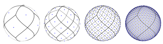
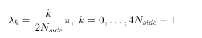
each base pixel is subdivided further into four equal area pixels. A HEALPix map therefore has N = 12N2 equal area (but di erently shaped) pixels, with the centers place don 4N side 1 ring of constant latitude. For any Nside, the HEAL Pixcenters,which wehen ceforth call the HEAL Pix points,arede nedal gebraically using three regions of the sphere, two polar (NandS)and one equatorial (E) [19]. Inspherical coordinates, the points in these regions are given as

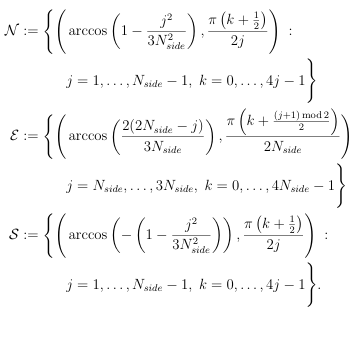
The nal HEALPix point set is X = N E S. The number of points on each ring varies in the polar regions, with only four points on the rings closest to the north and south poles of the sphere, whereas the rings in the equatorial region have the same number of points. This point distribution is illustrated more clearly in Figure 2.3, where the HEALPix points are displayed to a latitude-longitude grid. The biggest computational advantage for spherical harmonic analysis in the HEALPix scheme lies in the equally-spaced points on each ring of constant latitude. While this aides computation in the longitude direction with FFTs, the misaligned and unequally spaced points in latitude make fast bivariate Fourier analysis impossible without mod i cation. We address this in the new algorithm presented in section 2.3.

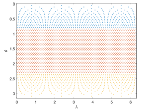
Figure 2.3 HEALPix grid on [0 2 ] [0 ], where is latitude, and is longitude. The point sets in the northern (N ), equatorial (E), and southern (S) regions are shown in blue, red, and yellow, respectively.

2.2.2 HEALPix Software Spherical Harmonic Analysis

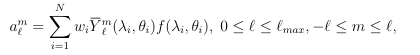
The standard method in the HEALPix software [10] for estimating the angular power spectrum (2.1) of data at the HEALPix points approximates the exact spherical harmonic coe cients (am) of the data as

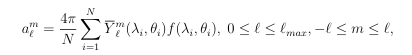
2.3

where ( i i) are HEALPix points in longitude-latitude, f is the data, and Ymis a spherical harmonic of degree and order m (see Appendix A for a discussion of the spherical harmonic conventions used in this paper). While the user can input any band limit max for this approximation, the software default is max = 3Nside 1. Due to the isolatitudinal nature of the HEALPix points, this computation is done with O(N3 2) complexity as opposed to O(N2) [11]. Note that N = O( 2 max), so the complexity of the amcomputation is equivalent to O( 3
max). The expression (2.3) is a low-order approximation to the continuous inner product (2.23) which de nes the coe cients, since it uses a simple equal weight quadrature. To improve this approximation, the software employs an iterative procedure, which is referred to as a Jacobi iteration [11]. In order to illustrate how the iterative method converges, we explain it below in the language of linear algebra.

The analysis operation, de ned in (2.3), produces an approximation to the spherical harmonic coe cients from the data f on the sphere, whereas the synthesis operation reconstructs the data given the spherical harmonic coefficients:

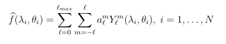
2.4

Note that we use a hat on f to indicate that computing the spherical harmonic coe cients according to (2.3) and using them in (2.4) gives di erent function values in general. In matrix-vector notation, we denote (2.3) and (2.4) as

Analysis: a = Af
Synthesis: f = Sa,
where a is the vector of spherical harmonic coe cients and f and f are the vectors of data values at the HEALPix points. Using this notation, the iterative procedure in the HEALPix software can be written as

r(k+1) = f Sa(k)
a(k+1) = a(k) + Ar(k+1),

2.5

where r is the residual vector and a(0) = Af. Substituting the rst equation of (2.5) into the last and using the fact that the analysis matrix satis es A = 4 N S, gives the iteration

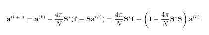
2.6

This is just stationary Richardson iteration (or Gradient Decent) with relaxation parameter 4N applied to the normal equations SSa = Sf [4, pp. 4445]. Thus, the iterative procedure converges to the least squares solution to (2.3), provided the spectral radius of I 4 N SS is less than one. The spectral radius also determines the convergence rate. Since the HEALPIx points are equidistributed, we know that (2.3) converges to the integral (2.23) as N (in exact arithmetic) [14]. Thus, the spectral radius of I 4 N SS converges to 0 as N and we expect the iteration (2.6) to converge more rapidly as N increases. Table 2.1 gives evidence of this result
by displaying the spectral radius of I 4N SS for increasing values of N.

Table 2.1 N.Spectral radius of the Richardson iteration matrix from (2.6) for different

values of

The default option in the HEALPix software sets the number of iterations of (2.6) to 3. While this does improve the accuracy of computing the spherical harmonic coe cients, it adds to the cost, as each iteration requires doing an analysis and synthesis ((2.3) and (2.4)) at a cost of O( 3 max) operations each. Since the solution converges to the least squares solution, one could improve the convergence of the Richardson iteration method by using algorithms like LSQR or conjugate gradient on the normal equations [27].

Pixel Weights and Ring Weights

As an alternative to the iterative scheme, the HEALPix software also has the option of using quadrature weights to improve the accuracy of the computation of the spherical harmonic coe cients. In this case, the equal weight quadrature approximation (2.3) is generalized to

2.7

where wi are the quadrature weights. There are two options for using quadrature weights. The rst is pixel weights , which uses di erent weights for each HEALPix point. These weights are computed using the positive quadrature weight algorithm from [19], which consists of solving a system involving a Gram matrix containing the spherical harmonics whose size is proportional to N [31]. For large N, the weights are computed once and stored. The second option is to use ring weights , which use di erent weights for each ring of the HEALPix point sets. The computation of the ring weights is done using similar ideas to the pixel weights, but a much smaller system has to be solved [31]. The new method introduced in this paper does not use quadrature weights directly, but instead computes the bivariate Fourier coe cients of the HEALPix data and then uses these to obtain the spherical harmonic coe cients.

2.3 HP2SPH

The algorithm presented here, named HP2SPH, introduces a new way to calculate the spherical harmonic coe cients of data sampled at the HEALPix points (2.2). The outline for the algorithm is given in Algorithm 1, and each of the pieces are described below.

2.3.1 Step1: Transform the data to a tensor product latitude longitude grid

As described in Section 2.2.1, the HEALPix grid has an unequal number of points on the rings in the northern (N) and southern (S) sets (2.2), and the points on the rings in the equatorial (E) set are shifted on every other ring. This structure leads to the pixels being misaligned in latitude. By upsampling the data on the northern and southern points in longitude so that there are an equivalent samples of the data Algorithm 1 HP2SPH
Input: Data sampled at the HEALPix point set of size N, fj , j = 1 Output: Approximate spherical harmonic coe cients, am , 0 m 1. Transform the data to a tensor product latitude-longitude grid: (i) N. max, Upsample the data in longitude from the northern (N) and southern (S) point sets using FFT (ii) Shift (interpolate) the data from the equatorial (E) point set so it is longi tudinally aligned 2. Compute the bivariate Fourier coe cients:
(i) Apply the DFS method (ii) Apply the inverse NUFFT-II in latitude (iii) Apply the inverse FFT in longitude
3. Obtain the spherical harmonic coe cients via the FSHT
on each ring and shifting the data at equatorial points in longitude, we can use fast algorithms to obtain the bivariate Fourier coe cients of the data as discussed in the next section. On the two polar point sets, we upsample the data using the trigonometric interpolant of the data on each ring of these sets to the non-shifted equally spaced longitude points on the equatorial rings, i.e.,

We also interpolate the data on the rings in the equatorial point set with shifted longitude points, to these values. Figure 2.4(b) illustrates the upsampling procedure leading to a tensor product latitude-longitude grid of data of size (4Nside 1) 4Nside. Wedescribe the interpolation procedure here for the data in the northern point set N. Consider the latitude values for the northern rings, j = arccos 1 j2 3N2 side j =

Figure 2.4 (a) HEALPix points with Nside = 16 displayed in latitude and longitude and (b) the corresponding upsampled points.

1……,Nside. We approximate the data in each ring using a trigonometric expansion of the form

The coe cients in the expansion are determined by enforcing interpolation of the given data values

With the minor algebraic manipulation of (2.9),

we see the interpolation conditions yield the system

2.10

which can be computed using the inverse FFT. We can then obtain the Fourier coef cients c(j) n in (2.9) for the data at the non-shifted values through simple multiplica tion3. Finally, we pad the vector containing the coe cients c(j) n with the appropriate number of zeros to get to a total of 4Nside, so that the expansion in longitude in each ring has the same number of Fourier coe cients. The values of the interpolant on each ring can then be obtained at the upsampled values (2.8) by applying the FFT on these padded vectors. A similar procedure can be applied to the data on the rings in the southern point set S. On the rings in the equatorial set E where the longitude values are shifted by (k + 1 2 ) (2Nside), we compute the Fourier coe cients of the data using (2.10) with j = Nside. We then obtain the coe cients in (2.9) at the non-shifted points from which the values can be computed using the FFT. No padding or upsampling is needed in this case.

2.3.2 Step 2: Compute Bivariate Fourier Coe cients

Bivariate Fourier analysis for data on the sphere requires the application of the DFS method to obtain periodicity of the data in latitude and to retain spherical symmetry. When we apply this method to the upsampled HEALPix data, there is an issue that the points in latitude are not equally-spaced, making the standard FFT unsuitable.
3Horners rule (and Estrins scheme for higher accuracy at small angles [7]) could also be used
to implement the shift, avoiding loss of accuracy due to evaluation of high frequency complex expo
nentials. To bypass this issue we use an NUFFT. Both the DFS technique and NUFFT method we use are discussed below for completeness.

Double Fourier Sphere (DFS) Method

A natural approach to representing a function on the sphere is to use a latitude longitude coordinate transform, de ned by x( ) =cos sin y( ) =sin sin z( )=cos ( ) [02 ] [0 ] (2.11) which maps the sphere to a rectangular domain. While this transformation allows for performing computations with the function f( ) = f(x( ) y( ) z( )), it also introduces arti cial boundaries at the north and south poles. In addition, the change of variables does not maintain the symmetry of functions on the sphere. Speci cally, the transform described in (2.11) does not preserve the periodicity in the latitude direction, which is necessary for bivariate Fourier analysis to be applicable and for results to make physical sense. These problems are solved by the DFS method. Originally introduced by Merilees in [23] (see also [40]) the DFS method transforms a function on the sphere to a rectangular grid while maintaining bi-periodicity. This can be thought of as doubling up the function f( ) to form a new function that preserves periodicity in both the latitude and longitude directions. Algebraically, this

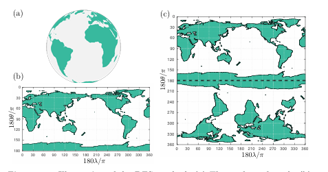
Figure 2.5 Illustration of the DFS method: (a) The surface of earth, (b) the surface mapped onto a latitude-longitude grid, and (c) the surface after applying the DFS method. [40]

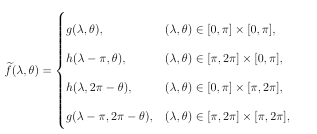
where g( )=f( )an dh( )=f( + )for( ) [0 ] [0 ].Figure 2.5 illustrates the DFS method applied to the surface of the Earth,which shows the preservation of bi-periodicity in(c).Wenotethat the DFS method canalsobeeasily applied to discrete data sample data tensor product latitude-longitude grid using (2.12),whichis what we do for the upsampled H E A L Pix data. In this case, (2.12)

corresponds to ipping and shifting the data matrix appropriately. Once the DFS method is applied to a function on the sphere, it can be approxi mated using a 2D bivariate Fourier expansion:

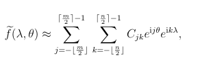
where m and n represent the number of frequencies in (doubled-up) latitude and longitude, respectively.
Note that the HEALPix grid does not include points at the north and south poles. When applying the DFS to the up sampled data from Step 1, this leads to a relatively large gap in the points in latitude over the poles compared to the other points, which can lead to issues with the inverse NUFFT (see below). To bypass this issue, we construct values at the two poles by using a weighted quadratic least squares t [8] that combines the data from the three rings closest to each pole. Remark.

The Fourier coe cients of the upsampled data in longitude are computed in Step 1. These can be used directly in the DFS procedure by applying (2.12) in Fourier space in the variable, which amounts to appending the (padded) coe cient matrix from Step 1 with a ipped version of itself with all odd wave numbers multiplied by 1. It then only remains to compute the Fourier coe cients in latitude to obtain the full bivariate Fourier coe cients. This is the focus of the next step.

Nonuniform Fast Fourier Transform (NUFFT)

The use of the nonuniform discrete Fourier transform (NUDFT) in many domain sciences has led to the development of algorithms for computing it e ciently. If these algorithms are quasi-optimal requiring O(nlogn), then they are referred to as a nonuniform fast Fourier transform (NUFFT). Given a vector c dimensional NUDFT computes the vector f Cn de ned by n 1

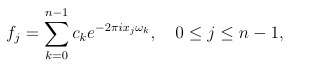
where xj [01]are the samples and k [0n]arethe frequencies. If the samples are equispaced (xj = j n) and the frequencies are integer ( k = k), then the the transform is a uniform DFT, which can be computed by the FFT in O(nlogn) operations [5]. When either the samples are nonequispaced or the frequencies are noninteger, the FFT does not directly apply without some careful manipulation [2]. Ruiz and Townsend [33] contributed to the collection of NUFFT algorithms by utilizing low rank matrix approximations to relate the NUDFT to the uniform DFT.

There are three types of NUDFTs and inverse NUDFTs that they account for in their algorithm: NUDFT-I, which has uniform samples but noninteger frequencies; NUDFT-II, which has nonuniform samples and integer frequencies; NUDFT-III, which has both nonuniform samples and nonuniform frequencies [12]. Since our HP2SPH method only uses the one-dimensional inverse NUFFT of the second type, we discuss the NUFFT-II algorithm [33]. Given Fourier coe cients, c Cn 1, the NUFFT-II attempts to approximate the vector

f = F2c 2.15

to machine precision in quasi-optimal complexity. Here (F2)jk = e 2 ixjk, xj are nonuniform samples (restricted to be in [01]), and k are integer frequencies for 0 <

jk n 1. Noticethat the DFT matrix for uniform samples and integer frequencies is similarly Fjk = e 2 ijk n. The key to the NUFFT-II algorithm described in [33] is that if the samples are nearly equispaced, then F2 can be related to the Hadamard product of F and a low rank matrix. This means that given a rank K approximation which relates F2 and F, the NUFFT-II can then be computed using K FFTs with O(Knlogn) cost. In practice, machine (double) precision can be achieved with K = 14 [33].

In the case of the inverse NUFFT-II, Ruiz and Townsend advocate for the use of the conjugate gradient (CG) method in order to solve the linear system F2c = f for c. Since F2 is not hermitian, the CG method is applied to the normal equations:

F2 F2c = F2f (2.16)

where F2 F2 is simply a Toeplitz matrix. Therefore, the inverse NUFFT-II can be cal culated using the CG method and a fast Toeplitz multiplication [9] in O(RCG nlogn) operations, where RCG is the number of CG iterations. The following suggestion is placed on the nonuniform function samples to avoid ill-conditioning in the system (2.16) [33]:

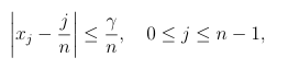
2.17

where 0 < 1 4. When this condition is satis ed, it has been experimentally observed that RCG
10 for a large range of n. For the method proposed in this paper, we apply the inverse NUFFT-II in latitude
to the DFS upsampled HEALPix data from Step 2. Unfortunately, the HEALPix points in latitude direction do not meet the condition (2.17). To bypass this issue, we instead use a least squares solution to compute fewer coe cients at the higher wave numbers than what the given data may support. We describe this procedure below
since it not discussed in [33].

The inverse NUFFT-II method computes rst column of the symmetric Toeplitz matrix F2 F2 in (2.16) in the following manner:

The last expression above can be computed e ciently by the NUFFT-I algorithm, since the NUDFT-I matrix is simply the transpose of the NUDFT-II matrix [33]. To compute a least squares solution to (2.15) with fewer coe cients, we simply truncate the rst column obtained from the above method to m < n terms and form the resulting m m Toeplitz matrix F2 F2. The right hand side for the least squares solution is obtained by similarly computing F2f and truncating this to m terms. For the DFS upsampled HEALPix data from Step 2, there are 8Nside coe cients in latitude, but only 4Nside coe cients in longitude.

To keep the number of Fourier modes in both directions (nearly) the same, we choose m = 4Nside+1 as the truncation parameter for the least squares solution for computing the Fourier coe cients in latitude. This is also a convenient choice since the method in step three for converting bivariate Fourier coe cients of data on the sphere to spherical harmonic coe cients requires the number of coe cients in each direction is the same and an odd number (we explain how to convert the coe cients in longitude to m = 4Nside+1 in the next
section). Remark. For problems where the data may contain noise (e.g., for the CMB ap –

plication), there could be an issue with this noise being ampli ed in steps 1 and 2. For step 1, we should not expect any additional noise to be introduced, since we are simply computing the Fourier coe cients on each ring using the original data and then shifting the coe cients and padding them with zeros. Step 2 has two areas where there could be an issue with noisy data. The rst is in constructing values at the poles and the second is in the application of the NUFFT in latitude. However, both of these steps apply a least squares procedure, which provides some smoothing. In our tests on CMB data, we did not observe any ampli cation of noise that was present in the data.

The HP2SPH method has a further bene t of using a backward stable algorithm for computing the spherical harmonic coe cients (as discussed next), which ensures that the resulting uncertainty in the spherical harmonic coe cients has only a low algebraic growth with respect to degree and is always proportional to the norm of the noise in the data.

2.3.3 Step 3: Obtain the spherical harmonic coefficients via the fast spherical harmonic transform (FSHT)

In [38], Slevinsky derives a fast, backward stable method for the transformation between spherical harmonic expansions and their bivariate Fourier series (given in (2.13)) by viewing it as a change of basis. This relation is defined as a connection problem, and the matrices that arise in the present case are well-conditioned, making them ideal for fast computations. Slevinsky describes the change of basis in two steps: con verting expansions in normalized associated Legendre functions to those of only order zero and one, and then re-expressing these in trigonometric form. In other words, it uses spherical harmonic expansions of order zero and one as intermediate expressions between higher-order spherical harmonics and their corresponding bivariate Fourier coefficients.

The rst step of the algorithm takes advantage of the fact that the matrix of connection coe cients between the associated Legendre functions of all orders and those of order zero and one can be represented by a product of Givens rotation matrices. This enables the use of the butter y algorithm, which can be thought of as an abstraction of the algebraic properties of fast Fourier transforms. The term butter y was introduced in [24], where it was used for analyzing scattering from electrically large surfaces, and then further developed in [26] for use in special function transforms.

Slevinsky uses the butter y algorithm to perform a factorization of the well-conditioned matrices of connection coe cients. The second step of this method exploits the hierarchical decompositions of the connection coe cient matrices between the associated Legendre functions of order zero and one to the Chebyshev polynomials of the rst and second kind, respectively. This step quickly computes the fast orthogonal polynomial transforms using an adap tation of the Fast Multipole Method [13] and low-rank matrix approximations. The total pre-computation time for both steps is O( 3 max log max), and execution time is asymptotically optimal with O( 2
max log2 max) operations. This FSHT is implemented in Julia with the package FastTransforms [37] (as are the NUFFT methods from [33] used in Step 2).

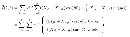
The FSHT in FastTransforms assumes the input function has a bivariate Fourier expansion of the form.

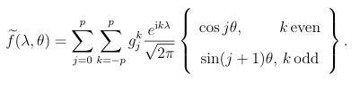
2.18

Any functionon the sphere is required tohave these even/oddconditions on its bivariateFouriercoe cients[23].At the end of step 2 we have obtained the bi variate Fourier expansion of the data of the form

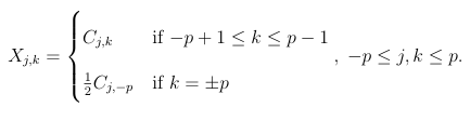
where p=N side 2. Since we are dealing with real-valued data,we can expand Fourier coe cientsarrayin to an odd number of points. The expanded array is defined by

Using the array X,we can write(2.19)as

from which we can obtain the coe cients g k j in(2.18). The F S H T software take sbivariate Fourier coefficients g k
j as input in anarray

organized as follows:

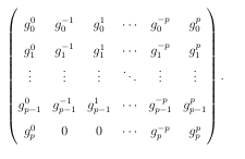
The out put of the software is the approximate spherical harmonic coefficients of the data arranged in anarray of the form

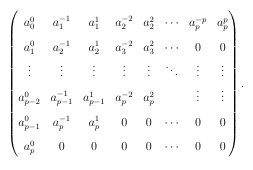
The angular power spectrum(2.1)can then be computed from this array.

2.4 Numerical Results

In this section we present a few numerical tests comparing the spherical harmonics and angular power spectrum(2.1) computed by our new method H P 2 S P H to the values computed by the HEALPix software employing the iterative scheme (2.6), pixel weights,and ring weights(2.7). The first test compares the rate at which the two methods converge to the spherical harmonic coefficients by applying them to deterministic (i.e. non noisy) functions sampled at the HEALPix points with know coeffi cients. The second test compares the accuracy of the methods using deterministic functions, which have a known power spectrum. In the third test, we compare the methods after calculating the angular power spectrum for a real CMB data map, which contains noise.

2.4.1 Convergence of Spherical Harmonic Coefficients

We choose the test function

where x( ) = [x( ) y( ) z( )] from (2.11) and the parameters, which we picked randomly, are given by

{ c1 ,c2, c3} = {5, 3,8}

{1 2 3 = 089149815815202726500042941346285753735997130328}
{1 2 3 = 12322175231079632059244524372349053779884082117}

The function (2 2x( ) x( c c))3 2 is a called a potential spline of order 3 2
centered at x( c c) and its exact spherical harmonic coe cients are given by [18]

aml= 18by ( l+5 /2) ( l+3/ 2) ( l+1 /2) ( l+1/ 2) (l+ 3/ 2) Yml( c, c)
(2.21)

These values are used to compare the convergence rates of the methods to the ex act spherical harmonic coe cients of f. We do this by plotting in Figure 2.6 the maximum absolute errors of the coe cients against the parameter t, which is used to determine the grid resolution parameter (Nside = 2t). Note that the spherical har monic coe cients of the CMB decay at a rate between O( 2) and O( 3) [39], which is slower than the decay rate of the coe cients of the test function (2.20) (since, for all m , Ym( c c) (2 +1) 4 , and the remaining terms in (2.21)
decay at a rate of O( 5)). This means that the test function has more smoothness than an actual CMB data set.

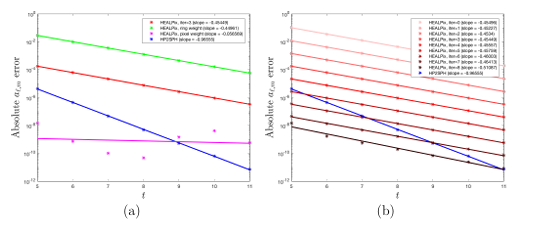
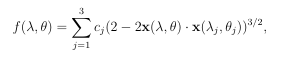
Figure 2.6 Maximum absolute errors as a function of t for the computed spherical harmonic coe cients of (2.20) using HP2SPH and (a) HEALPix (3 iterative re nement steps), pixel weights, ring weights and (b) HEALPix
with increasing iterative steps. The lines in the gure are the lines of best t to the data and the convergence rates are determined from the slope of this line (as displayed in the plot legends).

Figure 2.6(a) compares the four methods and shows that the HP2SPH method converges to the spherical harmonic coe cients of (2.20) at a rate at least twice as fast as any of the HEALPix methods. Although the consecutive iterative re nement steps used in the HEALPix method produce progressively better errors, Figure 2.6(b) illus trates that this does not improve the convergence rate (as discussed in Section 2.2.2). It is also important to note that after 8 iterative steps, there are no further improve ments in the accuracy, indicating the algorithm has nearly converged to the least squares solution to (2.3). The results the HEALPix method with pixel weights look pretty erratic with convergence achieved to 8-10 digits around t = 7, but no further reductions. This could be because of potential errors in the computed quadrature weights. Next, we test how the convergence rates of the methods are a ected by high frequencies. To do this we add 15 spherical harmonics to (2.20) with the following randomly chosen degrees and orders: The results from this test are displayed in

Figure 2.7 Maximum absolute errors as a function of t for the computed spherical harmonic coe cients of (2.20) augmented with spherical har monics using HP2SPH, HEALPix with 3 iterative re nement steps, pixel weights, and ring weights.

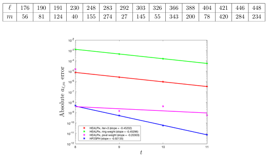
Figure 2.7. We note that in order to ensure the calculation of asymptotic convergence rates for all methods, we excluded the errors for t = 8 in the lines of best t. This test shows that the convergence rates of the new method as well as the iterative HEALPix scheme and the HEALPix method with ring weights are not a ected by the addition of high degree spherical harmonic terms to (2.20). The HEALPix method with pixel weights shows a similar erratic behavior to Figure 2.6(a), with no steady reductions in the errors after t = 9. The new HP2SPH method has the lowest errors of all the methods.

2.4.2 Errors in the Angular Power Spectrum

In this test, we rst explore the accuracy of all the methods for computing the angular power spectrum of (2.20). These results are compared to the exact spectrum, which is calculated using the exact spherical harmonic coefficients (2.21) in (2.1). The

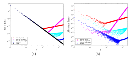
Figure 2.8 (a) Scaled angular power spectrum of (2.20) as a function of degree computed by the HEALPix software with 3 iterative re nement steps, the HP2SPH method, the HEALPix method with ring weights, and the HEALPix method with pixel weights. The exact power spectrum is given by the black s. Here Nside = 210, which is N = 12 582 912 total points. (b) Absolute errors in the (scaled) angular power spectrum of the results from (a) as a function of degree .

angular power spectrum of the four methods are displayed in Figure 2.8(a). We see that the algorithms produce similar results for lower degrees , but the HEALPix method with the iterative re nement scheme (2.6) diverges for degrees greater than approximately = 100, whereas the ring weight and pixel weight quadrature (2.7) results diverge for degrees greater than = 200. To compare the methods more directly, Figure 2.8(b) plots the absolute errors in the angular power spectrum for each degree . While the HEALPix method with ring weights performs the best out of all of the HEALPix methods for 50, the errors increase rapidly for higher .

Conversely, the HEALPix method with pixel weights does not perform as well for smaller , yet it performs better than the other HEALPix methods for larger . The HP2SPHmethod o ers comparable results for low as the pixel weights method while still maintaining accuracy for high .

Similar to Test 1, we test the accuracy of the methods when computing the power spectrum of data with high frequencies, as occur in real CMB data maps. As before, we add several spherical harmonic functions of high degree to the function (2.20). The new test function appends the following degrees and orders:

The power spectrum of this function is the same as (2.20), but with the value at each degree of appended spherical harmonics increased by 1 2+1 Figure 2.9(a) displays the errors in the angular power spectrum of this new function for all the methods over all , while Figure 2.9(b) displays the errors only over the range of that were appended to the base function. We again see that the ring weights provide the highest accuracy for low , but then the errors increase rapidly, while the HEALPix iterative method has the largest errors for low , but some of the

Figure 2.9 Absolute errors in the (scaled) angular power spectrum of (2.20) augmented with high-degree spherical harmonics computed by the HEALPix software with 3 iterative re nement steps, the HP2SPH method, the HEALPix method with ring weights, and the HEALPix method with pixel weights as a function of degree . (a) Displays the errors for degrees =
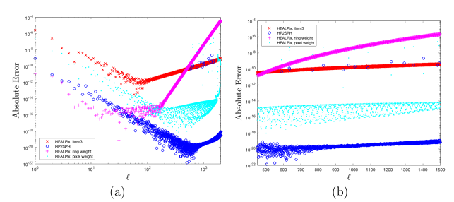
1 2000, while (b) displays the errors only for = 450 1500 to better show the how good the methods are at recovering the spectrum at the degrees of the appended spherical harmonics. Here Nside = 210, which is N = 12 582 912 total points.

smallest errors for the corresponding to the appended spherical harmonics. In contrast, the new HP2SPH method provides small errors over the entire angular power spectrum, clearly showing its bene ts over the HEALPix methods for determining the angular power spectrum of deterministic functions on the sphere.

2.4.3 Application to Real CMB Map

Our nal numerical test compares the methods on the real CMB map shown in Figure 2.1. Figure 2.10 (a) shows the angular power spectrum for this map computed with the methods, while (b) shows the errors in the three HEALPix methods com pared to the new HP2SPH method. We see from the gure that the new method (in blue) produces visually the same results as the HEALPix methods (red, magenta, and cyan), indicating that the new method is not anymore susceptible to noise than the HEALPix methods.

Figure 2.10 (Scaled) angular power spectrum of the CMB data map dis played in Figure 2.1 (a) with Nside = 211 for the four methods discussed in the paper (left), and the relative errors of the HEALPix software methods against the HP2SPH method (right).

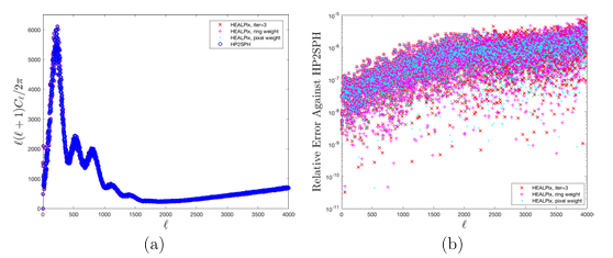
2.5 Conclusions and Remarks

We have presented a new method, HP2SPH, for performing discrete spherical harmonic analysis on data collected using the HEALPix scheme. The method utilizes the FFT, NUFFT, and the FSHT to compute the spherical harmonic transform in near optimal computational complexity (O(N log2 N) complexity for N total HEALPix points). Several numerical tests were presented to demonstrate the improved convergence and accuracy of the new method relative to the various HEALPix approaches for problems involving synthetic data with no noise, except that introduced by round o errors. In the case of a real CMB map with additional types of noise, the power spectra computed by the methods show good agreement. The new HP2SPH bene ts further from the backward stability of the FSHT, which ensures that the resulting uncertainty in the spherical harmonic coe cients has only a low algebraic growth with respect to degree and is always proportional to the norm of the noise in the data.

We anticipate the new method will be applicable to the many other areas where the HEALPIx scheme is used and is naturally generalizable to other equal-area isolatitudinal sampling schemes for the sphere. For our next steps, we will work to optimize the implementation of the method, which is currently in Julia, to improve its actual run-time. This will include transcribing our code into a lower-level language like C; e orts in this direction are already
underway for the FSHT [36]. In addition to this, we will include the ability to perform Fourier synthesis on a CMB map, i.e. given an angular power spectrum, we will return the corresponding CMB map values. For this purpose, our method has another advantage over HEALPix in that we will have the bivariate Fourier coe cients, which will simply make the synthesis an application of the FFT and NUFFT. Finally, we plan to add functionality for analyzing the polarization of CMB maps.

Acknowledgements

We are grateful to Ann Almgren for her comments and suggestions as well as Richard Mikael Slevinsky for assisting us with using the FastTransforms package. We also thank the entire HEALPix team, especially Kris Gorski and Martin Reinecke, for their feedback and assistance on this work. Finally, we thank the anonymous re viewers whose comments helped improve the paper. The rst authors work was supported by the SMART Scholarship, which is funded by The Under Secretary of Defense-Research and Engineering, National Defense Education Program / BA-1, Basic Research. The second authors work was supported by National Science Foun dation grant CCF 1717556.

Appendix A: Spherical Harmonic Conventions

We denote a scalar spherical harmonico fdegree 0 andorder m as Y m( ),where is the azimuthang leand is the zenith angle.We denethese functionsas

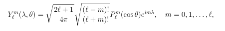
where Ym=( 1)mYm form<0andPm(cos )are the associate Legendre functions. As eigenfunctions of the Laplace Beltrami operator, spherical harmonics are
the natural basis for square integrable functions on the sphere [1]. Inother words,
any L 2-integrable function f on the sphere can be unique lyre presented as

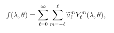
where the spherical harmonic coe cients, am, are found using the usual L 2-inner product for scalar functions on the sphere:

REFERENCES

[1] K. Atkinson and W. Han. Spherical Harmonics and Approximations on the Unit Sphere: An Introduction. Springer Berlin Heidelberg, 2012.

[2] R. Beatson and L. Greengard. A short course on fast multipole methods. Wavelets Multilevel Methods elliptic PDEs, 1:137, 1997.

[3] C. L. Bennett, D. Larson, J. L. Weiland, N. Jarosik, G. Hinshaw, N. Odegard, K. M. Smith, R. S. Hill, B. Gold, M. Halpern, E. Komatsu, M. R. Nolta, L. Page, D. N. Spergel, E. Wollack, J. Dunkley, A. Kogut, M. Limon, S. S. Meyer, G. S. Tucker, and E. L. Wright. Nine-year Wilkinson Microwave Anisotropy Probe (WMAP) Observations: Final Maps and Results. The Astrophysical Journal Supplement Series, 208(2):20, 2013.

[4] M. Benzi, G. H. Golub, and J. Liesen. Numerical solution of saddle point prob lems. Acta Numerica, 14(1):1137, 2005.

[5] J. Cooley and J. Tukey. An algorithm for the machine calculation of complex Fourier series. Math. Comp., 19:297301, 1965.

[6] R. G. Crittenden and N. G. Turok. Exactly azimuthal pixelizations of the sky. Technical Report DAMTP-1998-78, University of Cambridge, 1998. astro ph/9806374.

[7] G. Estrin. Organization of computer systems the xed plus variable structure computer. In Proc. Western Joint IREAIEE-ACM Comput. Conf., pages 3340, 1960.

[8] G. E. Fasshauer. Matrix Approximation Methods with MATLAB. World Scienti c Publishers, Singapore, 2007.

[9] G. Golub and C. F. Van Loan. Matrix Computations. Johns Hopkins University Press, Baltimore, 1996.

[10] K. M. Gorski, B. D. Wandelt, E. Hivon, F. K. Hansen, and A. J. Banday. The HEALPix Primer. arXivpreprint astro-ph/9905275, 1999.

[11] K. M. Gorski, B. D. Wandelt, E. Hivon, F. K. Hansen, A. J. Banday, M. Reinecke, and M. Bartelmann. HEALPix A framework for high resolution discretization, and fast analysis of data distributed on the sphere. ApJ., 622:759771, 2005.

[12] L. Greengard and J. Lee. Accelerating the nonuniform fast Fourier transform. SIAM Rev., 46:443454, 2004.

[13] L. Greengard and V. Rokhlin. A fast algorithm for particle simulations. J. Comp. Phys., 73:325348, 1987.

[14] D. P. Hardin, T. Michaels, and E. B. Sa . A comparison of popular point con gurations on S2. Dolomites Res. Notes Approx., 9:1649, 2016.

[15] G. Hinshaw, D. Larson, E. Komatsu, D. N. Spergel, C. L. Bennett, J. Dunkley, M. R. Nolta, M. Halpern, R. S. Hill, N. Odegard, L. Page, K. M. Smith, J. L. Weiland, B. Gold, N. Jarosik, A. Kogut, M. Limon, S. S. Meyer, G. S. Tucker,

E. Wollack, and E. L. Wright. Nine-year Wilkinson Microwave Anisotropy Probe (WMAP) Observations: Cosmological Results. The Astrophysical Journal Sup plement Series, 208(2):19, 2013.

[16] R. C. Hoover, A. A. Maciejewski, and R. G. Roberts. Pose detection of 3-D objects using S2-correlated images and discrete spherical harmonic transforms. In 2008 IEEE International Conference on Robotics and Automation, pages 993 998, 2008.

[17] W. Hu and S. Dodelson. Cosmic microwave background anisotropies. Ann. Rev. Astron. Astrophys., 40:171216, 2002.

[18] S. Hubbert and B. J. C. Baxter. Radial basis functions for the sphere. In Recent progress in multivariate approximation (Witten-Bommerholz, 2000), volume 137 of Internat. Ser. Numer. Math., pages 3347. Birkhauser, Basel, 2001.

[19] J. Keiner and D. Potts. Fast evaluation of quadrature formulae on the sphere. Math. Comp., 77:397419, 2008.

[20] P. Leopardi. A partition of the unit sphere into regions of equal area and small diameter. Electron. Trans. Numer. Anal., 25:309327, 2006.

[21] C. Majeau, E. Agol, and N. B. Cowan. A two-dimensional infrared map of the extrasolar planet HD 189733b. The Astrophysical Journal, 747(2):L20, 2012.

[22] Z. Malkin. A new equal-area isolatitudinal grid on a spherical surface. The Astronomical Journal, 158(4):158, 2019.

[23] P. E. Merilees. The pseudospectral approximation applied to the shallow water equations on a sphere. Atmosphere, 11:1320, 1973.

[24] E. Michielssen and A. Boag. A multilevel matrix decomposition algorithm for analyzing scattering from large structures. IEEE Trans. Antennas and Propaga tion, 44:10861093, 1996.

[25] R. S. Miller, G. Nerurkar, and D. J. Lawrence. Enhanced hydrogen at the lunar poles: New insights from the detection of epithermal and fast neutron signatures. Journal of Geophysical Research: Planets, 117(E11), 2012.

[26] M. ONeil, F. Woolfe, and V. Rokhlin. An algorithm for the rapid evaluation of special function transforms. Appl. Comput. Harmon. Anal., 28:203226, 2010.

[27] C. C. Paige and M. A. Saunders. LSQR: An algorithm for sparse linear equations and sparse least squares. ACM Trans. Math. Softw., 8(1):4371, 1982.

[28] P. Paykari and J.-L. Starck. CMB data analysis. Advances in Machine Learning and Data Mining for Astronomy, pages 5587, 2012.

[29] W. J. Percival, S. Cole, D. J. Eisenstein, R. C. Nichol, J. A. Peacock, A. C. Pope, and A.S. Szalay. Measuring the Baryon Acoustic Oscillation scale using the Sloan Digital Sky Survey and 2dF Galaxy Redshift Survey. MNRAS, 381(3):1053 1066, 10 2007.

[30] Planck Collaboration 2005. Planck: The scienti c programme. ESA publication ESA-SCI(2005)/01, 2005.

[31] M. Reinecke. personal communication, June 5, 2019.

[32] C. Roecker, N. S. Bowden, G. Carosi, M. He ner, and I. Jovanovic. Recon struction algorithms for directional neutron detection using a time projection chamber. Nuclear Technology, 180(2):231240, 2012.

[33] D. Ruiz-Antoln and A. Townsend. A nonuniform fast Fourier transform based on low rank approximation. SIAM J. Sci. Comput., 40:A529A547, 2018.

[34] E. B. Sa and A. B. J. Kuijlaars. Distributing many points on a sphere. Math. Intelligencer, 19:511, 1997.

[35] L. P. Singer and L. R. Price. Rapid Bayesian position reconstruction for gravitational-wave transients. Phys. Rev. D, 93:024013, Jan 2016.

[36] R. M.Slevinsky. FastTransforms. https://github.com/MikaelSlevinsky/FastTransforms. GitHub.

[37] R. M.Slevinsky. FastTransforms.jl. https://github.com/MikaelSlevinsky/FastTransforms.jl. GitHub.

[38] R. M. Slevinsky. Fast and backward stable transforms between spherical har monic expansions and bivariate fourier series. Appl. Comput. Harmon. Anal., 47:585606, 2019.

[39] J.-L. Starck, M. J. Fadili, and A. Rassat. Low-CMB analysis and inpainting. Astronomy and Astrophysics, 550, Jan 2013. [40] A. Townsend, H. Wilber, and G. B. Wright. Computing with functions in spher ical and polar geometries I. the sphere. SIAM Journal on Scienti c Computing, 38(4):C403C425, 2016.

[41] D. R. Weimer, E. K. Sutton, M. G. Mlynczak, and L. A. Hunt. Intercalibration of neutral density measurements for mapping the thermosphere. Journal of Geophysical Research: Space Physics, 121(6):59755990, 2016.

[42] M. White. Anisotropies in the CMB. Proceedings of Division of Particles and Fields of the American Physical Society, 1999.

CHAPTER 3:

A DIVERGENCE-FREE AND CURL-FREE RADIAL BASIS FUNCTION PARTITION OF
UNITY METHOD

Kathryn P. Drake, Edward J. Fuselier, and Grady B. Wright
arXiv:2010.15898, 2020.1

Abstract

Divergence-free (div-free) and curl-free vector elds are pervasive in many areas of science and engineering, from uid dynamics to electromagnetism. A common problem that arises in applications is that of constructing smooth approximants to these vector elds and/or their potentials based only on dis crete samples. Additionally, it is often necessary that the vector approximants preserve the div-free or curl-free properties of the eld to maintain certain physical constraints. Div/curl-free radial basis functions (RBFs) are a particularly good choice for this application as they are meshfree and analytically satisfy the div-free or curl-free property. However, this method can be computationally expensive due to its global nature. In this paper, we develop a technique for 1Submitted for publication in the SIAM Journal of Scienti c Computing.

bypassing this issue that combines div/curl-free RBFs in a partition of unity framework, where one solves for local approximants over subsets of the global samples and then blends them together to form a div-free or curl-free global approximant. The method is applicable to div/curl-free vector elds in R2 and tangential elds on two-dimensional surfaces, such as the sphere, and the curl-free method can be generalized to vector elds in Rd. The method also pro duces an approximant for the scalar potential of the underlying sampled eld. We present error estimates and demonstrate the e ectiveness of the method on several test problems.

3.1 Introduction

Approximating vector elds from scattered samples is a pervasive problem in many scienti c applications, including, for example, uid dynamics, meteorology, magnetohy dro dynamics, electromagnetics, gravitational lensing, imaging, and computer graphics. Often these vector elds have certain di erential invariant properties relatedto an underlying physical principle. For example, in incompressible uid dynamics the velocity of the uid is divergence-free (div-free) as a consequence of the conservation of mass. Similarly, in electromagnetics the electric eld is curl-free in the absence of a time varying magnetic eld as a consequence of the conservation of energy. Addition ally, the elds may have properties of being tangential to a surface (e.g., the sphere S2) and have a corresponding surface div-free or curl-free property, as occurs in many areas of geophysical sciences [15]. In several of these applications it is necessary for the approximants to preserve these di erential invariants to maintain certain physical constraints. For example, in incompressible ow simulations using the immersed

Approximating vector elds from scattered samples is a pervasive problem in many scienti c applications, including, for example, uid dynamics, meteorology, mag netohydrodynamics, electromagnetics, gravitational lensing, imaging, and computer graphics. Often these vector elds have certain di erential invariant properties related to an underlying physical principle. For example, in incompressible uid dynamics the velocity of the uid is divergence-free (div-free) as a consequence of the conservation of mass. Similarly, in electromagnetics the electric eld is curl-free in the absence of a time varying magnetic eld as a consequence of the conservation of energy. Addition ally, the elds may have properties of being tangential to a surface (e.g., the sphere S2) and have a corresponding surface div-free or curl-free property, as occurs in many areas of geophysical sciences [15]. In several of these applications it is necessary for the approximants to preserve these di erential invariants to maintain certain physical constraints. For example, in incompressible ow simulations using the immersed

domain. Additionally, each evaluation of the resulting interpolant involves dN terms. If the div/curl-free RBFs are constructed from scalar-valued RBFs with global support, then the linear system is dense and not well suited to iterative methods. To ameliorate these issues, a multilevel framework has been developed for compactly sup ported div/curl-free RBFs in [16]. However, we take a di erent approach to reducing the computational cost using the partition of unity method (PUM) [31, 43, 17, 6, 30]. In RBF-PUM, one only needs to solve for local approximants over small subsets of the global data set and then blend them together to form a smooth global approx imant.

A particular challenge with extending this idea to div/curl-free RBFs is in enforcing that the global approximant is analytically div/curl-free. To overcome this challenge, we use the local div/curl-free RBFs to obtain local approximants to scalar potentials for the eld and then blend these together to form a global scalar potential for the entire eld. A div/curl-free vector approximant is then obtained by applying the appropriate di erential operator to the global scalar potential. The method as presented here will only work for elds that can be de ned by scalar potentials, which includes div/curl-free vector elds in R2, surface div/curl-free tangential elds on two-dimensional surfaces, and curl-free elds in Rd, but not div-free elds in R3. However, there are several bene ts of the method. First, for node sets X that are qua siuniform, the algorithm parameters can be chosen to produce global approximants to the eld in O(N logN) operations. Second, we have error estimates showing the method can give high rates of convergence, and numerical evidence that rates faster than algebraic with increasing N are possible. Unlike the method from [16], these convergence rates are possible with the xed complexity of O(N logN). Finally, a global approximant for the scalar potential is given directly from the samples withouthaving to compute derivatives of the sampled eld or solving a Poisson problem.

Asfar as weare aware, the only other computationally scalable div-free approxima tion technique for scattered data is the div-free moving least squares (MLS) method from [42]. The method is used for generating nite di erence type discretizations for Stokes equations. While it worked quite successfully for this application, it can be computationally expensive for more general approximation problems, since it re quires solving a new (small) linear system for each evaluation point. For the method we develop, the (small) linear systems are independent of the evaluation points.

The rest of the paper is organized as follows. In the next section we introduce some background material necessary for the presentation of the method. Section 3 contains a review of PUM and then presents the div/curl-free RBF-PUM. Error estimates for the new method are presented in Section 4. Section 5 contains numerical experiments demonstrating the convergence rates of the method on three model problems. The nal section contains some concluding remarks.

3.2 Div/Curl-free RBFs

We review the generalized vector RBF techniques for reconstructing vector elds below, rst for div-free elds and then for curl-free elds. In both cases, we focus on approximations of tangential vector elds on smooth, orientable, surfaces embedded in R3 (which includes R2 and S2). In the curl-free case the method extends trivially to Rd. Before discussing these two techniques, we introduce some notation and review some relevant background material.

3.2.1 Notation and preliminaries

Let P denote a smooth, orientable surface embedded in R3, possibly with a boundary, and let n R3 denote the unit normal vector to P expressed in the Cartesian basis. When discussing tangential vector elds on P, we use the terms divergence and curl to be tacitly understood to refer to surface divergence and surface curl for P. The surface curl (or rot) operator L and the surface gradient operator G play a central role in de ning div-free and curl-free tangential elds on P. We can express these operators in extrinsic (Cartesian) coordinates as follows:

L =n G=(I nnT)

where is the standard R3 gradient, and I is the 3-by-3 identity matrix. It is well-known that div-free and curl-free elds are locally images of these operators. Proposition. Let u be a tangential vector eld de ned on P then
1. u is div-free if and only if locally there exists a scalar potential : P such that u = L( )R
2. u is curl-free if and only if locally there exists a scalar potential : P such that u = G(l )R
Both potentials are unique up to the addition of a constant.

The method in this paper relies on the fact that the elds involved have scalar po tentials that are unique up to a constant. Three dimensional div-free vector elds have vector potentials unique up to the addition of the gradient of a harmonic scalar function, and it is not clear how our method might carry to that case. However, it

will be applicable to curl-free field since higher dimensions since a vector field u on Rd is curl-free if and only if u= for some scalar potential. In what proceeds,we use the following notation for the L operator:

3.1

where n=(a 1 a 2 a 3)is the unit normal to P at x.Note that applying Q x to a vector in R 3 gives the cross product of n with that vector. Similarly,we express G as

3.2

where Px=I nnT projects any vector at x on Pin to a planet angent to P a t x. Two important cases of Pare P=R 2 and P=S 2. For the former case, the unit normal is independent of its position and is typically chosen as n=(001). Using this with(3.1)and(3.2), leads to the standard definition for these operators for vector fields on R 2:

which can be truncated to remove the unnecessary third component .For P=S 2,the unit normal at x is n=x,but L and G do not simplify beyond this.

3.2.2 Div-free RBF interpolation

Div-free vector RB F interpolants are similar to scalar R BF interpolants in the sense that one constructs them from linear combinations of shifts of a kernel at each of the given data sites. The difference between the approaches is that in the vector case one uses a matrix-valued kernel whose columns are div-free. For the sake of brevity, we give the nal construction of these kernels and refer to reader to [35] for a rigorous derivation. For more information on scalar-valued RBFs, which we do not discuss here, see any of the books [17, 44, 19].
Let : R3 R3 Rbearadial kernel in the sense that (xy) = ( x y ), for some : [0 ) R, where is the vector 2-norm. It is common in this case to simply write (xy) = ( x y ). Supposing has two continuous derivatives, then the matrix kernel div is constructed using the operator L in (3.1) as

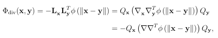
where the subscripts in the di erential operators indicate which variables they operate on and, for simplicity, no subscript means they operate on the x component. Here we have used the fact that the matrix Qx in (3.1) is skew-symmetric and T y ( x y ) = T ( x y ). For any c R3 and xed y P, the vector eld div(xy)c is tangent to P and div-free in x, which follows from Proposition 3.2.1 since

The second argument of div acts as a shift of the kernel and indicates where the field divc is centered.
An interpolant to a div-free tangential vector eld u : P R3 sampled at distinct points X = xj N j=1 P can be constructed using div as follows:

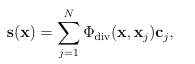
3.6

where the coe cients cj j=1 div(xxj)cj R3 are tangent to P at xj (this is necessary to make the interpolation problem well-posed as discussed below) and are chosen so that sX =uX .We refer to (3.6) as a div-free RBF interpolant.
Instinctively, one may try to solve for the expansion coe cients in (3.6) by im posing s(xj) = uj, j = 1
N, where uj = u(xj). However, this will lead to a singular system of equations since each uj can be expressed using only two degrees of freedom rather than three. To remedy this, let dj ej nj be orthonormal vectors at the node xj, where nj is the outward normal to P, ej is a unit tangent vector to P, and dj = nj ej. Since uj is tangent to P we can write it in this basis as uj = jdj+ jej, where j = dT juj and j = eT juj. We may also express each tangent cj as cj = jdj + jej, which leads us to express (3.6) as

s(x) =n j=1 div(xxj)[ jdj + jej]

3.7

and to write the interpolation conditions as dT i s(xi) = i and eT i s(xi) = i. This leads to the 2 N-by-2 N system of equations

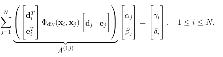
The interpolation matrix that arises from this system(with its(i j)t h 2-by-2 block given by A(ij))is positive definite if div is constructed from an appropriately chosen scalar-valued R BF(e.g.,a positive definite )[35].
When P=R2, the div-free RBF interpolant can be simplified considerably since in this case we can choose dj=(100)and ej=(010)and use(3.3) for defining div. Using this in(3.7) and truncating the unnecessary third component of the vector interpolant(sinceit is always zero)gives the expansion

s(x)=sumof N j=1 div(xxj)cj

3.9

wheres cj R2,and

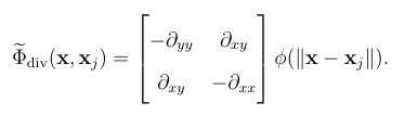
This expression for div can be written as div = I + T , which is the standard way to express div-free kernels for general Rd [22]. An important consequence from the construction of the div-free RBF interpolant (3.6)is that we can extract ascalarpotential for the interpolated eld. Using(3.5) for div in (3.6) we have

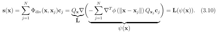
This potential will play a crucial role in the developing the PUM in Section 3.3

3.2.3 Curl-free RBF interpolation

Curl-free vector RBF interpolants are constructed in a similar fashion to the div-free ones, the only di erence being that G is applied instead of L in the construction of the matrix kernel. Given a scalar RBF and using a derivation similar to (3.4), curl is given as

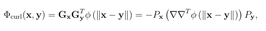
3.11

where we have used the fact that the Px matrix in (3.2) is symmetric. For any c R3 and xed y P, the vector eld curl(xy)c is tangential to P and curl-free in x. This follows from Proposition 3.2.1 since

3.12

As with the div-free kernel (3.5), the second argument of curl acts as a shift of the kernel and indicates where the eld curlc is centered . Interpolants to a curl-free tangential vector eld u : P R3 sampled at distinct points X = xj N
j=1 P are constructed from curl as

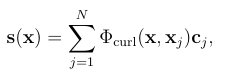
3.13

where the coe cients cj R3 are tangent to P at xj and are chosen so that sX = uX .The procedure for determining these coe cients is identical to the div-free case, one just needs to replace div with curl in (3.7) & (3.8). The matrix from the linear system (3.8) with curl is similarly positive de nite for the same . Further, a scalar potential can also be extracted from the curl-free eld (3.13) using (4.2):

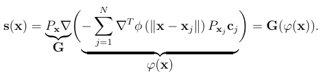
3.14

In the Euclidean case Rd, the curl-free kernel is simply given as curl(xy) = T ( x y ) [22], where is the d-dimensional gradient. The interpolation conditions sX= uX also lead to the simpli ed linear system for the expansion coe cients cj Rd:

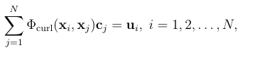
sum ofNj=empty set 1curl(xi xj)cj = ui i = 12N

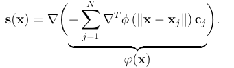
3.3 A div-free/curl-free partition of unity method

The cost associated with solving the linear systems (3.8) and (3.15) is O(N3), which is prohibitively high when the number of nodes N in X is large. In this section, we develop a partition of unity method (PUM) that requires solving several linear systems associated with subsets X of X with n << N nodes, which reduces the computational cost signi cantly regardless of the nature of the RBF used.

3.3.1 Partition of unity methods

Letf : Rd be an open, bounded domain of interest for approximating some function R. Let 1 M be a collection of distinct overlapping patches that form an open cover of , i.e., M=1 , and let the overlap between patches be limited such that at most K << M patches overlap at any given point x For each = 1 M, let w :. [01] be a weight function such that w is compactly supported on that M =1 w and the set of weight functions w have the property 1. Suppose s is some approximation to f on each patch . The partition of unity approach of Babuska and Melenk [3] is to form an approximant s to f over the whole domain by blending the local approximants s with w via
s = M =1 ws. When samples of f are given at N scattered nodes X = xj N j=1 , RBF interpolants are a natural choice for the local approximants s, as pointed out in [3].

RBF-PUM was rst explored for interpolation in 2002 by Wendland [43] and Lazzaro and Montefusco [31], and then later in 2007 by Fasshauer [17, Ch. 29]. More recent work has explored various aspects of the method in terms of applications, methods, and implementations, especially by Cavoretto, De Rossi, and colleagues (e.g., [7, 8, 9]), and also extensions to problems on the sphere [6, 40]. Additionally, the method has been adapted for approximating the solution of partial di erential equations (e.g., [38, 41, 30, 1]).

Commonchoices for the patches in RBF-PUM are disks for problems in R2, spherical caps for problems on S2, and balls for problems in R3, and these are the choices we use throughout this paper. Figure 3.1 gives an example of a set of patches for a problem in R2. Techniques for choosing the patches are discussed in, e.g., [9, 30, 40]
(see Section 3.3.3 for more discussion). Based on the choices of patches, the weight functions w can be constructed using Shepards method as follows. Let : R+ R have compact support over the interval [01). For each patch , let denote its center and denote its radius, and de ne (x) := ( x). The weight functions are then given by

wl(x)=kl(x)/ sum of mj=1 kj(x),l=1,…..m.

Note that each w is only supported over and that the summation on the bottomonly involves terms that are non-zero over patch , which is bounded by K. Figure 3.1 (b) illustrates one of these weights functions for the example domain in part (a), where is chosen as the C1 quadratic B-spline

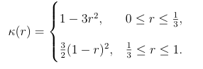
This is the weight function we use throughout the paper.

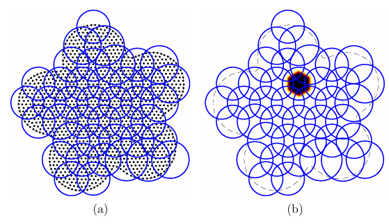
Figure 3.1 (a) Illustration of partition of unity patches (outlined in blue lines) for a node set X (marked with black disks) contained in a domain (marked with a dashed line). (b) Illustration of one of the PU weight
functions for the patches from part (a), where the color transition from white to yellow to red to black correspond to weight function values from 0 to 1.

3.3.2 Description of the method

A rst approach at a vector RBF-PUM may be to construct local vector approximantss for the patches
that make up the PU using either (3.6) for div-free elds or (3.13) for curl-free elds. These approximants can then be blended into a global approximant for the underlying field:

s =M=sum of l1 wl sl

3.18

The issue with this approach is that s will not necessarily inherit the div-free or curl-free properties of s because of the multiplication by the weight functions w. We instead use the local scalar potentials that are recovered from each s and then blend those together. A div-free or curl-free approximant can then be recovered by applying the appropriate di erential operator to the blended potentials. Since the essential ingredients are very similar for all the kernels treated from Section 3.2, for brevity we describe the method only for the div-free case in R2 and mention any relevant di erences as needed.

Let Xdenote the nodes from X R2 that belong to patch , and let s denote the div-free RBF interpolant (3.6) to the target div-free eld u over X. Our interest is also in the scalar potential for each interpolant given in (3.10), which we denote as . While we could try to construct a global PU approximant for the scalar potential of the eld and then apply the operator L to the result, we would immediately run into problems since the scalar potentials are only unique up to a constant. This means that for two patches and k that overlap, and k could be o up to
the addition of a constant in the overlap region and thus lead to an inaccurate PU approximant. To rectify this situation, we need to shift each such that +b k +bk if and k overlap.

To summarize, the main steps of the div-free PUM are as follows:

1. On each patch , compute a divergence free interpolant x and extract its

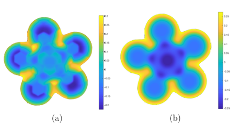
Figure 3.2 Div-free RBF partition of unity approximant of the potential from Section 3.5.1 (a) without the patch potentials shifted ( k) (b) with the patch potentials shifted ( k).

scalar potential using (3.10).

2. Determine constants b M=1 such that := +bk= .k +bk =: k whenever

3. Blend the shifted potentials with the PU weight functions to obtain a global approximant for the underlying potential:

3.19

4. Apply L to to obtain a global div-free approximant to the underlying field:

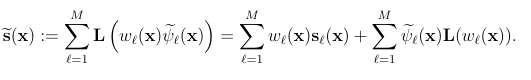
3.20

Note that the second term in the last equality acts as a correction to the PU approx imant formed by just blending the div-free RBF interpolants. Figure 3.2 illustrates the necessity of shifting the patch potentials by way of an example from Section 3.5.1.
The gure shows a div-free RBF-PU approximant of a potential when the local patch potentials are not shifted (i.e., using shifted. in (3.19) rather than ) and when they are
We now turn our attention to determining the constants b M =1 for shifting the potential. If and k overlap, then let xkdenote the center of the overlap region: xk := ( k + k) ( k+ ), where < k to avoid redundancy; see Figure 3.3 for an illustration. We refer to these points at the glue points since they are where

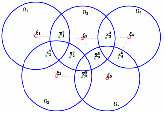
Figure 3.3 Illustration of the glue points for shifting the potentials. The asterisks denote the glue points and the small circles denote the patch centers.

we will glue the potentials between neighboring patches to each other. We denote the collection of all such points by X := xk k = < k = xi i L =1, where L = X and we have reindexed the set so that each xi = xk for some unique overlapping pair of patches and k. On this set we want to impose the conditions (xk) + b = k(xk) + bk for some constants b, = 1M, which we refer to as the potential shifts . This can be arranged into a sparse L-by-M over-determined linear system

Pb =c 3.21

with the following properties. The L-by-M matrix P is sparse with two non-zeros per row: the ith row, where xi corresponds to xk, has a 1 in the th column and a 1 in the kth column. The vector b contains the potential shifts, and the vector c is given by ci = k(xi) (xi) = k(xk) (xk). The matrix P also has rank M 1. This follows since P is the (oriented) incidence matrix for the graph with vertices being the patch centers and edges corresponding to non-empty intersections of patches. Based on the assumption that M =1 is an overlapping open covering, this graph is
connected, so rank(P) = M 1 [12, Thm. 10.5]. In the next section we discuss the procedure we use to determine the potential shifts from (3.21). Remark. The procedure described above works exactly the same for curl-free elds in R2 and R3 using (4.6) for the interpolants and potential elds on each patch. The procedure also extends to more general surfaces P for div-free elds (using (3.10)) and curl-free elds (using (3.14)). However, in this case determining the glue points can be more di cult, but for P = S2, this is trivial.

3.3.3 Implementation details

We now discuss how the patches M=1 are chosen as well as how one might compute the potential shifts from the system (3.21). In what follows, we assume that the nodes X are quasiuniformly distributed (i.e., have low discrepancy) in the underlying domain , so that the mesh-norm for X,

h := sup min dist (x,y),y xy

satis es h = O(1 dN), where d is the dimension of . We also assume that there is a signed distance function for the domain to distinguish the interior from the exterior.

Patch centers

To determine the patches for domains in R2 and R3, we use an approach similar to the one described in [30]. The idea is to start with a regular grid structure of spacing H that covers the domain of interest and then remove the grid points that are not contained in the domain. The remaining grid points are chosen as the patch centers M M =1. Next, an initial radius is chosen proportional to H so the patches =1 form an open cover and there is su cient overlap between patches (speci cs on this are given below). Finally, for any node in X that is not contained in one of the patches, the nearest patch center j is determined and the radius j for that patch is enlarged to enclose the node. We perform all range queries on patch centers using a k-d tree.

For domains in R2, we choose the initial grid structure for the patch centers as regular hexagonal lattice of spacing H. Neighboring patches will not overlap if the initial radius is less than or equal to H2. Therefore, to guarantee overlap, we set the initial radii for the patches to = (1+ )H2, where > 0. See Figure 3.1 for an illustration of the patches chosen using this algorithm for = 1 2. For domains in R3, we choose the initial grid structure for the patch centers as a regular Cartesian lattice of spacing H. In this case, neighboring patches along the longest diagonal directions will not overlap if the initial radius is less than or equal to 3H2. To guarantee overlap, we thus set the initial radii for the patches to = (1 + ) 3H2.

To determine the patches for S2, we use an approach similar to the one described in [40]. The idea is to use M quasi-uniformly spaced points on S2 for the set of patch centers. We choose these as near minimum energy (ME) point sets [28], and use the pre-computed near ones from [46]. For a set with M points, the average spacing H between the points can be estimated as H 4 M. Weselect a value of H and then determine M as M = 4 H2 . Since the ME points are typically arranged in hexagonal patterns (with a few exceptions [28]), we choose the radius for each patch as =(1+ )H2, where the parameter again determines the overlap. To keep the overall cost under control, the initial radii of the patches H should decrease as N increases. The rate at which H should decrease can be determined as follows.

Assuming that the patches that intersect the boundary have similar radii to the interior patches, and using the assumption that X is quasiuniform, a simple volume argument gives that number of nodes in each patch satis es n = O( dN) = O(HdN), where d is the dimension of . So, to keep the work roughly constant per patch, we need H = O(1N1 d). In our implementation of the vector PUM, we choose

H =q(AN)1 d 3.23

where A is related to the area/volume of , and q is a parameter that controls the average number of nodes per patch. Note that from the above analysis, the compu tational cost increases as the overlap parameter increases and as q increases. Based on the assumptions on X and the patches, choosing H according to (3.23) results in a computational cost of O(N) for constructing the vector PUM approximants,

and O(N logN) for the range queries involved for determining the patch structure. However, in practice, the cost is dominated by the former part of the method.

Potential shifts

Since rank(P) = M 1 and its nullspace consists of constant vectors, we rst set one of the shifts bj to zero, for some 1 j M, and then compute the remaining shifts using the least squares solution of (3.21). For this problem we can form the normal equations directly since the matrix PTP is just a graph Laplacian (recall P is an oriented incidence matrix). We have found that the accuracy of the reconstructed field (3.20) can often be improved if a weighted least squares approach is used. In this case, we use a diagonal weight matrix W with entries that depend on the distance between the glue points and the patch centers. Speci cally, we set ri as the closer of the two distances between the ith glue point xi and the centers of the two patches it was formed from, and then set

where rmin = minj rj and > 0. The normal equations in this case now look like a weighted graph Laplacian.

3.4 Error Estimates

The error bounds will be expressed in terms of local mesh norms h, which are given by (3.22), with = and X = X. Error rates for RBF interpolation, including divergence-free (curl-free) RBF approximation, both in at space and on the sphere, have been known for some time. Many of these estimates are valid for target functions within the native space, which we denote by N( ), of the RBF used- which for innitely smooth RBFs are subspaces of analytic functions and for kernels of nite smoothness are essentially Sobolev spaces (with norms equivalent to Sobolev norms
on bounded subsets)2. For the RBF kernels considered here, there is a continuous
embedding from the native space into a Sobolev space of order > d2. In this
situation we get the estimate below.

Proposition.

Suppose that u N( ) and that each satisfies an interior cone condition with angle independent of . Then there is a constant C independent of diam( ) such that

||u s L|| ( ) <CE(h l)||u N||( l) ,

where E(h) = h d2 for some > d2 if the kernel has nite smoothness, andE(h) 0 faster than any xed h if the kernel is innitely smooth. Proof. Estimates like these have been worked out for div/curl-free RBFs on subsets of Rd and on S2 [22, 23, 25]. We should however address that in the papers referenced the domain was xed- but here the size of the domain should scale with h, so we should brie y review why the constant C does not depend on the size of the domain. First, note that the function u s will be zero on X. On domains satifying an interior cone condition, in the Euclidean case and on surfaces, we may therefore 2See [44, Ch. 10] for native spaces of scalar valued functions, and see [21, 23] for the vector cases on Rd and the sphere. employ a zeros lemma in each coordinate function to get3 inequalities of the form:

||u s L ||l(l ) <Chl t-dby2|| u s H||( l),

where H( )denotes the space of tangent vector fields with each coordinate function in the Sobolev space H( ). In these results, the constant only depends on the domain by way of the angle of an interior cone condition, i.e., C depends on the geometry of the domain and not its size [27, Theorems A.4 and A.11]. Next, since u N( ), then u N( ) and there is an isometric extension E : N( ) N( )suchthat EuN( ) = uN( ) (see[44, Theorem10.46,10.47]4). With this, since N( ) is continously embedded in H( ) for some > d2, we get u s H( ) = Eu sEu H( ) Eu sEu H( ) CEu sEu N( ) where we write sEu = s to emphasize that the interpolant on Xof the extension is also s. Note that the constant here may depend on , but not on . Finally, it is
well-known that the interpolation error is always orthogonal to the kernel interpolant
in the native space, which implies the bound

||Eu- sEul|| N<||( ) Eu||N=( )=|| u||N( )

where the last equality follows because E is an isometry. This completes the proof. In addition to the estimate above, our arguments that follow will also rely on the
3See, for example, the Appendix in [27]
4The theorems referenced are given in the Euclidean scalar-valued context, but the arguments
are general enouch to apply to matrix valued positive de nite kernels on any set.

Mean Value Theorem, which for a scalar function and xy Rd we express as

where x is on the line segment between x and y. Here we use the notation to denote the Euclidean length when the argument is a vector. To derive a similar estimate on surfaces, let xy P and let : [0distP(xy)] P denote a shortest
path in P connecting x and y with (0) = x, (distP(xy)) = y, parameterized by arclength. This implies that
is tangent to P and variable Mean Value Theorem to the real-valued function = 1. Applying the single implies that

where t [0distP(xy)]. Since is tangent to P and has length 1, we get =
G G . Combining the above with the fact that G( ) = L( ) gives us the following

where x P.

Before proceeding we summarize some of the important assumptions on the partition of unity. Recall that each x
is covered by only a small number of patches (say at most K patches). We also assume that the number of patches that intersect a given patch is uniformly bounded by some constant m. Additionally, we suppose that there are roughly the same number of nodes in each patch, and that the node

distribution in each patch is quasi-uniform. This leads to an estimate of the formch diam( ) Ch for some constants cC independent of . Lastly, we assume that the partition is 1-stable (see [44][Def. 15.16]), meaning that rst order deriva tives of the weight functions satisfy a bound of the form w C(diam( )) 1, where C is some constant independent of . This with the quasi-uniformity supposition gives the bound w = Lw Ch 1 for some C independent of .

Now we give an estimate for the point wise error of the divergence-free approximant in a two dimensional domain. Note that the bound is local in the sense that it comprised of a local interpolation error plus an expression involving the residuals rk := (xk) k(xk) from adjusting neighboring potential functions. Theorem 1. Given a div-free vector eld u = L( ) N( ), let and s = L( ) denote the PUM approximants from (3.19) and (3.20). Then the error at x satisfies

where k is any index such that x.
Proof. The rst equality follows from the fact that Gf and Lf have the same magnitude. Next, note that

The rst term is a weighted average of RBF interpolants to u and the weight functions sum to 1,so we have

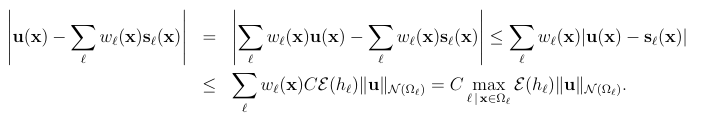
To complete the proof we need to bound these condtermin(3.27).Given x ,x ak such that x k. Since L(w)=0 and w(x)=0 for x we get

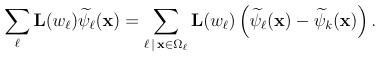
This and our assumptions on the weight functions give us the estimate

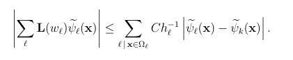
If l=k,the corresponding term in the sum is zero. If =k,we let g:= k and x k be the adjustment point for and k,we can rewrite

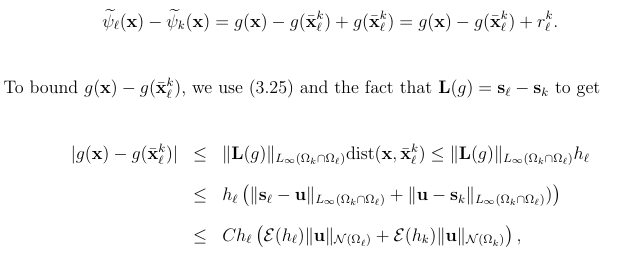
which when applied to(3.28)gives

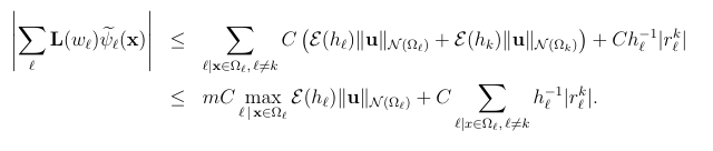
The result follows.

Note that very similar arguments follow through also for curl-free vector field son surfaces, i.e. an estimate identical to(3.26)holds for the curl-free case. The proof also carries directly over to Rd-namelyifu= ,ands= denotes the curl-free RBF-PUM approximant , one has an estimate of the form

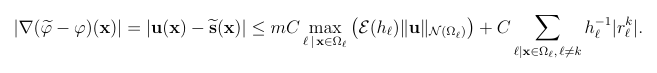
Now we discuss the residual in shifting the local potentials. We begin by showing that good constants for the shifts exist. Proposition.Let s =L be the local RBF interpolanton X and let X= X be the collection of glue point son . Given any v such that u=L(v), the constant

gives

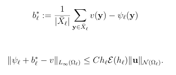
Proof. Letx .First we apply the triangle in equality and the Mean Value The o rem to obtain

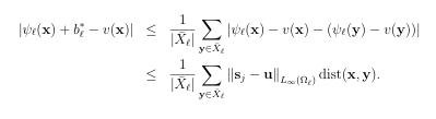
Next, an application of Proposition 3.4 and the fact that diam( ) Ch nishes the proof. Letting r := Pb c, i.e., the residual in the system (3.21) using the shifts given in the above proposition, with a triangle inequality and using the fact that hk h for neighboring patches, we get

3.29

Applying this to the residual term from (3.26) becomes:

3.30

Thus if the shifts are chosen appropriately the method can achieve the same approximation order as that of local interpolation. However, we compute the shifts according to the over determined (3.21). The residual from that system satis es the following. Proposition. Let b be the least squares solution to (3.21). The residual r := Pb c satis es the bound

Proof. Choose any scalar potential v such that u = L(v), and let b be the vector whose th element is b as de ned in Proposition 3.4. Then we have r we square the left-most inequality in (3.29) and estimate further to get

3.31

Now sum the estimate over all glue points, and note that each (and k) will appear in the sum at most m times (the maximum number of patches that intersect any given patch). This gives the result. In an attempt to bound the error solely in terms of the point distribution and target function, let us look at an application of this estimate to the residual term from (3.26). For simplicity, assume that all h h for all h. Since there are at most mterms in the sum, a Cauchy-Schwarz inequality gives

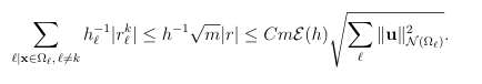
Due to the sum over all patches, this bound may or may not match the expected error rates. A very rough estimate would introduce a factor of M, where M is the number of patches. In the quasi-uniform case, a volume argument gives M h d2.

Thus a worst-case scenario is that the method converges according to E(h)h d2. However, numerical experiments suggest that the errors decay according to E(h) (see for example Section 3.5.2) and do not seem to depend on the number of patches which suggests that the estimate E(h)h d2 is pessimistic. We conjecture that the correct error rate is indeed E(h).

3.5 Numerical experiments

In this section, we numerically study the vector RBF-PUM for three di erent test problems: a div-free eld in a star-shaped domain in R2, a div-free eld on S2, and a curl-free eld in the unit ball in R3. For each of these cases, we numerically test the convergence rates of the method and compare them to the estimates from Section 3.4. The point sets we use in the experiments are all quasiuniform, so rather than compute the mesh-norm h and use this to measure convergence rates, we simply use h N 1d. To illustrate the di erent convergence rates that are possible, we use the inverse multiquadric (IMQ) kernel (r) = 1 1+( r)2 and the Matern kernel (r) = e r 1+( r)+ 3
7 ( r)2 + 2 21 ( r)3 + 1 105 ( r)4 . The latter kernel is piecewise smooth and the local error from Proposition 3.4, in terms of N, is given by E(N) = ( N) 35 for d = 2 (see [25] for more details). The IMQ kernel is analytic and therefore the local error decreases faster than any algebraic rate. For scalar interpolation with the IMQ, the local error estimate is E(N) = e Clog(N)N1 2d [37], where C > 0 is a con stant. We demonstrate that this also appears to be the correct rate for the vectorcase. While the error estimates are in terms the-norm, we also include results on the 2-norm for comparison purposes. Since we are interested in demonstrating the convergence rates from the theory, we x the shape parameter in all the tests, as using di erent on a per patch level will lead to di erent constants in the estimates. The values were selected so that conditioning of the linear systems (3.8) (or (3.15)) is not an issue. Choosing variable shape parameters in scalar RBF-PUM is explored in [10] and may be adapted to the current method, but we leave that to a separate study. For brevity we report results for one kernel per example, with the IMQ ker nel used for the rst and third test and the Matern used for the second. However,

we note that the estimated convergence rates for each kernel were consistent with the theory across all tests. Finally, we set the weighted least squares parameter in (3.24) to = 4. This value produced good results over all the numerical experiments performed.

All results were obtained from a MATLAB implementation of the vector RBF PU M method executed on a Mac Book Pro with an Intel i 7 dual-core 3.5 GHzprocessor and 16 GB RAM. No explicit parallelization was implemented.

3.5.1 Div-free eld on R2

The target field and domain for this numerical test are de ned as follows. Let the potential for the field be

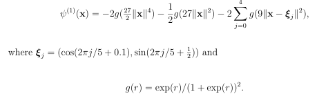
(3.32) (3.33)

The target domain is set from the potential as (1) = x R2 (1)(x) target div-free vector eld is u(1)110, and
div = L (1). This gives a star-like domain with a non trivial eld that is tangential to and field. ; see Figure 3.4 for a visualization of the potential The node sets X for this test were initially generated from DistMesh [36], but
then perturbed by a small amount to remove any regular structures. The sizes of the node sets for the tests are N = 11149, 17405, 30943, 44570, and 69635. We

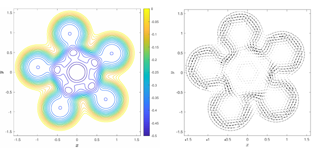
Figure 3.4 Contours of the potential (1) (left) and corresponding div-free velocity eld u (1) div (right) for the numerical experiment on R2

estimate A in (3.23) to be 6, and use an overlap parameter for the patches of = 1 2. We test three di erent values of q to see how the errors are e ected by increasing the nodes per patch. For q = 6810, there are an average of 63112173 nodes per patch, respectively. The boundaries create some variability in the nodes per patch and lead to minimum values of 325785 and the maximums of 109191300, respectively. As mentioned above, we only report results for the IMQ kernel, for which the shape parameter is set to = 13 for all tests. Errors in the approximations of the target potential and eld are computed at a dense set of 94252 points over the domain. Errors in the approximation of the target potential are computed after rst normalizing the approximant and the potential to have a mean of zero over the evaluation points. For each N and q, the error reported is the average of the-norm (2-norm) errors using 20 di erent random perturbations of the initial node set X. This reduces large spreads in the errors caused by particularly good and bad samples of the target eld. Figure 3.5 displays the relative-norm and 2-norm errors in the approximation

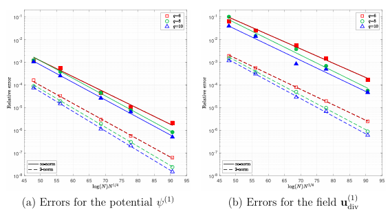
Figure 3.5 Convergence results for the numerical experiment on the star domain in R2 for the IMQ kernel and di erent values of q. Filled (open) markers correspond to the relative -norm (2-norm) errors and solid (dashed) lines indicate the t to the estimate E(N) = e C log(N)N1 4 , with-out the rst values included.

of the target potential and eld as a function of log(N)N14. Included in the gures are the lines of best t to the errors using the error estimate E(N) = e C log(N)N1 4 from scalar RBF theory. We see from the gure that this error estimate provides a good t to both the -norm and 2-norm errors for the potential and the eld. The -norm errors for the potential have more variability especially for q = 6, but the 2-norm errors are quite consistent. As expected, the errors in reconstructing the potential are lower than those for reconstructing the eld, and the 2-norm errors are lower than the -norm errors. Increasing q leads to a consistent decrease in the 2-norm errors, but the decrease is more variable for the -norm errors.

3.5.2 Div-free eldonS2

Letx=(xy z) S2,and the potential for the target field be defined as

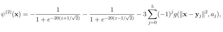
where g is given in(3.33),yj=(cos( j)cos( j) sin( j)cos( j) sin( j))for j 5 j=0= 005,11,212,318,422,526 and j 5
j=0=079 082,076, 081,08, 077 ,and aj=4+j 2. The div-free fieldis the n given as u(2)
div=L (2). The value s use din (3.34)were chosen to produce a zonal jet in the mid-latitudes with three superim posed vortices in each of the northern and southern hemispheres;see Figure 3.6 fora visualization of the potentialand field.

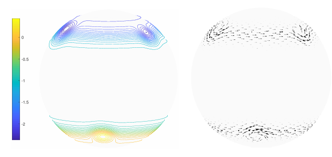
Figure 3.6 Contours of the potential (2) (left) and corresponding div-free velocity eldu(2) div(right)for the numerical experiment on S2.

The node sets X for this test are chosen as Hammersley nodes,which give quasi uniform,but random sampling points for S2 [46]. The sizes of the nodesets for the test sare N=10000,15000,20000,30000,40000,50000 and 60000. Weuse A=4 in(3.23)and set the over lap parameter to =9 16. We again use three different

Figure 3.7 Convergence rates for the numerical experiment on S2 for the Matern kernel and di erent values of q. Filled (open) markers correspond to the relative -norm (2-norm) errors and solid (dashed) lines indicate the lines of best t to the -norm (2-norm) errors as a function of N on a loglog scale. The legend indicates the slopes of these lines with the rst number corresponding to the -norm and the second the 2-norm, which give estimates for the algebraic convergence rates

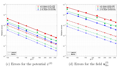
values of q to see how the errors are e ected by increasing the nodes per patch. For q = 6 9 12, there are an average of 63 143 252 nodes per patch, respectively. Since there are no boundaries for this domain, the number of nodes per patch is much more consistent across all patches. The minimum nodes per patch are 58 137 245 and the maximums are 69 150 261, respective to the q values. For this example, we only re port results for the Matern kernel, for which the shape parameter is set to = 75 for all tests. Errors in the approximations of the target potential and eld are computed at a quasiuniform set of 92163 points over S2. Errors in the approximation of the target potential are again computed after rst normalizing the approximant and the potential to have a mean of zero over the evaluation points. Similar to the previous experiment, for each N and q, the error reported is the average of the-norm (2 norm) errors from 20 different random rotations of the initial Ham mersley node set

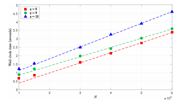
Figure 3.8 Timing results for the numerical experiment on S2 with di fferent values of q. The dashed lines are the lines of best t to the timings using all but the rst two values.

Figure 3.7 displays the relative -norm and 2-norm errors in the approximation of the target potential and eld as a function of N12. Included in the gure are the lines of best t to the log of the errors vs. the log of N12 for each q, and the slopes of these lines are reported in the legend of the gure (where the rst number is for -norm and second for the 2-norm). We see from this gure that the computed rates of convergence for the -norm are slightly higher than the theoretical rate of 35.

Thus the residual estimate from Proposition 3.4 is not leading to a reduction in the convergence rates as discussed at the end of Section 3.4. We also see from the gure that the estimated rates for the 2-norm errors are higher than the -norm errors as one would expect. Finally, similar to the previous experiment, we see that the errors in reconstructing the potential are lower than those for reconstructing the field. We also display the timing results for this experiment in Figure 3.8 for running the entire algorithm with 20164 evaluation points. We see from the data and the corresponding lines of best t that the complexity appears to be O(N). The predicted O(N logN) complexity is most likely not visible over the range of N considered.

3.5.3 Curl-free eld on the unit ball

The target curl-free eld for this test is generated as follows. Let g(ra) = (a+r2) 1 2 and de ne the following potential:

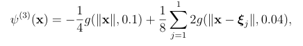
where xj 12 j=1 are the vertices of a regular icosahedron with each vertex a distance
of 2/3 from the origin. The target curl-free is then generated by u(3) curl = (3).

This eld can be interpreted as the (idealized) electric eld that is generated from a negative (smoothed) point charge at the origin, surrounded by 12 positive (smoothed) point charges, equidistance from one another; see Figure 3.9(a) for a visualization of the potential and field.

The node sets X for this test are obtained from the meshfree node generator described in [39], which produces quasiuniform but unstructured nodes in general domains; see Figure 3.9 (b) for an example of the nodes used for the unit ball. The sizes of the node sets for the tests are N = 4999, 9103, 19636, 59116, and 158474.

We use A =4 3 in(3.23) and an overlap parameter of = 1 4. We again test three different values of q: q = 234. For q = 2, the minimum, average, and maximum nodes per patch are 18, 37, 83, for q = 3 these values are 72, 120, 238, and for q = 4 these values are 186, 271, 512. As with the rst experiment, we only present

Figure 3.9 (a) Visualization of the potential (3) and corresponding curl free velocity eld u(3) =
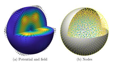
curl (3) for the numerical experiment on the unit ball. (b) Example of N = 4999 node set (small solid disks) used in the nu merical experiment on the unit ball, where colors of the nodes are propor tional to their distance from the origin (yellow=1, green = 0.5, blue=0). The
plots in both gures show the unit ball with a wedge removed to aid in the visualization.

results for the IMQ kernel, for which the shape parameter is set to = 4 for all tests. Errors in the approximations of the target potential and eld are computed at a set of 208707 points over the unit ball. Errors in the approximation of the target potential are again computed after rst normalizing the approximant and the potential to have a mean of zero over the evaluation points. Similar to the previous experiments, for each N and q, the error reported is the average of the -norm (2-norm) errors from 20 di erent random rotations of the initial node set X. Figure 3.10 displays the relative -norm and 2-norm errors in the approximation of the target potential and eld as a function of log(N)N16. As in the rst experiment, we have included the lines of best t to the errors, but now using E(N) = e C log(N)N1 6 . We see from the Figure that the error estimate again gen

Figure 3.10 Convergence results for the numerical experiment on the unit ball in R3 for the IMQ kernel and di erent values of q. Filled (open) mark ers correspond to the relative -norm (2-norm) errors and solid (dashed) lines indicate the t to the expected error estimate E(N) = e C log(N)N1 6 , without the rst values included.

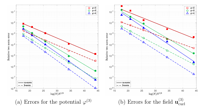
erally provides a good t to both the -norm and 2-norm errors for the potential and the field. The -norm errors deviate more from the estimates than the 2-norm errors, especially for eld in the q = 2 case. However, for this case the minimum number of points per patch can be quite small.

3.6 Concluding remarks

We have presented a new method based on div/curl-free RBFs and PUM for approx imating div/curl-free vector elds in R2 and S2, and for curl-free elds in R3. The method produces approximants that are analytically div/curl-free and also produces an approximant potential for the eld at no additional cost. For quasi-uniform samples, we have shown how the parameters can be selected so that the computational complexity of the method is O(N log N). We have proved error estimates for the approximants based on local estimates for the div/curl-free interpolants on the PU patches. We have also demonstrated the high-order convergence rates of the method on three di erent test problems with samples ranging from thousands to hundreds of thousands of nodes all done on a standard laptop.

While we have only focused on div/curl-free interpolation over local patches, a future area to explore is to instead use a least squares approach similar to the one used for scalar RBFs in [30]. Here one can choose fewer centers in the local patches for the div/curl-free RBFs than data samples, a technique referred to as regression splines in the statistics literature [17, ch. 19]. This has the bene t of further reducing the cost of the local patch solves for the approximation coe cients and could provide some regularization. Another future area to explore is the adaption of stable algorithms for at RBFs [20, 18] to the div/curl-free RBFs.

These algorithms are especially important in scalar RBF-PUM methods based on smooth RBFs for reaching high
accuracies [30]. Some work has been done along these lines for S2 in [14], but not for the local setting on patches. A nal promising area for future research is in developing adaptive algorithms for the method along the lines of [10].

Acknowledgments

We thank Elisabeth Larsson for helpful discussions regarding the PU patch distribution algorithm and Varun Shankar for generating the node sets used for the unit ball example. KPDs work was partially supported by the SMART Scholarship funded by The Under Secretary of Defense-Research and Engineering, National Defense Eucation Program/BA-1, Basic Research. GBWs work was partially supported by National Science Foundation grant 1717556.

REFERENCES

[1] K. A. Aiton. A Radial Basis Function Partition of Unity Method for Transport on the Sphere. Masters thesis, Boise State University, USA, 2014.

[2] L. Amodei and M. N. Benbourhim. A vector spline approximation. J. Approx. Theory, 67(1):5179, 1991.

[3] I. Babuska and J. M. Melenk. The partition of unity method. Int. J. Numer. Meths. Eng., 40:727758, 1997.

[4] Y. Bao, A. Donev, B. E. Gri th, D. M. McQueen, andC.S.Peskin. An immersed boundary method with divergence-free velocity interpolation and force spreading.

J. Comput. Phys., 347:183206, 2017.

[5] H. Bhatia, G. Norgard, V. Pascucci, and P.-T. Bremer. The Helmholtz-Hodge decomposition a survey. IEEE Transactions on Visualization and Computer Graphics, 19(8):13861404, 2013.

[6] R. Cavoretto and A. De Rossi. Fast and accurate interpolation of large scattered data sets on the sphere. Comput. Appl. Math., pages 15051521, 2010.

[7] R. Cavoretto and A. De Rossi. A trivariate interpolation algorithm using a cube-partition searching procedure. SIAM J. Sci. Comput., 37(4):A1891A1908, 2015.

[8] R. Cavoretto, A. De Rossi, G. E. Fasshauer, M. J. McCourt, and E. Perrac chione. Anisotropic weights for RBF-PU interpolation with subdomains of vari able shapes. In Radu F., Kumar K., Berre I., Nordbotten J., Pop I. (eds) Numerical Mathematics and Advanced Applications ENUMATH 2017. Lecture Notes in Computational Science and Engineering. Springer, Cham, 2019.

[9] R. Cavoretto, A. De Rossi, and E. Perracchione. Partition of unity inter polation on multivariate convex domains. Int. J. Model. Simul. Sci. Comp., 06(04):1550034, 2015.

[10] R. Cavoretto, A. De Rossi, and E. Perracchione. RBF-PU interpolation with variable subdomain sizes and shape parameters. In AIP Conference Proceedings, volume 1776, page 070003. AIP Publishing, 2016.

[11] D. Coe, E. Fuselier, N. Bentez, T. Broadhurst, B. Frye, and H. Ford. LensPer fect: Gravitational lens mass map reconstructions yielding exact reproduction of all multiple images. Astrophys. J, 681(2):814830, 2008.

[12] A. Dharwadker and S. Pirzad. Graph Theory. CreateSpace Independent Pub lishing Platform, North Charleston, SC, USA, 2011.

[13] F. Dodu and C. Rabut. Irrotational or divergence-free interpolation. Numer. Math., 98(3):477498, 2004.

[14] K. P. Drake and G. B. Wright. A stable algorithm for divergence-free radial basis functions in the at limit. J. Comput. Phys., 417:109595, 2020.

[15] M. Fan, D. Paul, T. C. M. Lee, and T. Matsuo. Modeling tangential vector fields on a sphere. Journal of the American Statistical Association, 113(524):1625 1636, 2018.

[16] P. Farrell, K. Gillow, and H. Wendland. Multilevel interpolation of divergence free vector elds. IMA J. Numer. Anal., 37(1):332353, 2016.

[17] G. E. Fasshauer. Meshfree Approximation Methods with MATLAB, Interdisciplinary Mathematical Sciences. World Scienti c Publishers, Singapore, 2007.

[18] G. E. Fasshauer and M. J. McCourt. Stable evaluation of Gaussian radial basis function interpolants. SIAM J. Sci. Comput., 34:A737A762, 2012.

[19] B. Fornberg and N. Flyer. A Primer on Radial Basis Functions with Applications to the Geosciences. SIAM, Philadelphia, 2014.

[20] B. Fornberg, E. Larsson, and N. Flyer. Stable computations with Gaussian radial basis functions. SIAM J. Sci. Comput., 33:869892, 2011.

[21] E. J. Fuselier. Improved stability estimates and a characterization of the native space for matrix-valued RBFs. Adv. Comput. Math., 29(3):269290, 2008.

[22] E. J. Fuselier. Sobolev-type approximation rates for divergence-free and curl-free RBF interpolants. Math. Comp., 77(263):14071423, 2008.

[23] E. J. Fuselier, F. J. Narcowich, J. D. Ward, and G. B. Wright. Error and stability estimates for surface-divergence free RBF interpolants on the sphere. Math. Comp., 78(268):21572186, 2009.

[24] E. J. Fuselier, V. Shankar, and G. B. Wright. A high-order radial basis function (RBF) Leray projection method for the solution of the incompressible unsteady Stokes equations. Comput. Fluids, 128:4152, 2016.

[25] E. J. Fuselier and G. B. Wright. Stability and error estimates for vector eld interpolation and decomposition on the sphere with RBFs. SIAM J. Numer. Anal., 47(5):32133239, 2009.

[26] D. Handscomb. Local recovery of a solenoidal vector eld by an extension of the thin-plate spline technique. Numer. Algorithms, 5(1-4):121129, 1993. Algorithms for approximation, III (Oxford, 1992).

[27] T. Hangelbroek, F. J. Narcowich, and J. D. Ward. Polyharmonic and related kernels on manifolds: Interpolation and approximation. Foundations of Computational Mathematics, 12(5):625670, Jan. 2012.

[28] D. P. Hardin and E. B. Sa . Discretizing manifolds via minimum energy points. Notices Amer. Math. Soc., 51:11861194, 2004.

[29] U. Harlander, T. von Larcher, G. B. Wright, M. Ho , K. Alexandrov, and C. Eg bers. Orthogonal decomposition methods to analyze PIV, LDA and thermog raphy data of a thermally driven rotating annulus laboratory experiment. In T. von Larcher and P. D. Williams, editors, Modelling Atmospheric and Oceanic ows: insights from laboratory experiments and numerical simulations. American Geophysical Union, Washington D.C., 2014.

[30] E. Larsson, V. Shcherbakov, and A. Heryudono. A least squares radial basis function partition of unity method for solving PDEs. SIAM J. Sci. Comput., 39(6):A2538A2563, 2017.

[31] D. Lazzaro and L. B. Montefusco. Radial basis functions for the multivariate interpolation of large scattered data sets. J. Comp. Appl. Math., 140(1):521536, 2002.

[32] S. Lowitzsch. Error estimates for matrix-valued radial basis function interpolation. J. Approx. Theory, 137:238249, 2005.

[33] A. A. Mitrano and R. B. Platte. A numerical study of divergence-free kernel approximations. Appl. Numer. Math., 96:94 107, 2015.

[34] F. J. Narcowich and J. D. Ward. Generalized Hermite interpolation via matrix valued conditionally positive de nite functions. Math. Comp., 63(208):661687, 1994.

[35] F. J. Narcowich, J. D. Ward, and G. B. Wright. Divergence-free RBFs on surfaces. J. Fourier Anal. Appl., 13:643663, 2007.

[36] P.-O. Persson and G. Strang. A simple mesh generator in Matlab. SIAM Rev., 46(2):329345, 2004.

[37] C. Rieger and B. Zwicknagl. Sampling inequalities for innitely smooth functions, with applications to interpolation and machine learning. Adv. Comput. Math., 32(1):103129, 2010.

[38] A. Safdari-Vaighani, A. Heryudono, and E. Larsson. A radial basis function partition of unity collocation method for convectiondi usion equations arising in nancial applications. J. Sci. Comput., 64(2):341367, 2015.

[39] V. Shankar, R. Kirby, and A. Fogelson. Robust node generation for mesh-free dis cretizations on irregular domains and surfaces. SIAM J. Sci. Comput., 40:A2584 A2608, 2018.

[40] V. Shankar and G. B. Wright. Mesh-free semi-Lagrangian methods for transport on a sphere using radial basis functions. J. Comput. Phys., 366:170190, Aug. 2018.

[41] V. Shcherbakov. Radial basis function partition of unity operator splitting method for pricing multi-asset American options. BIT, 56(4):14011423, 2016.

[42] N. Trask, M. Maxey, and X. Hu. A compatible high-order meshless method for the Stokes equations with applications to suspension ows. J. Comput. Phys., 355:310326, 2018.

[43] H. Wendland. Fast evaluation of radial basis functions : Methods based on partition of unity. In Approximation Theory X: Wavelets, Splines, and Applications, pages 473483. Vanderbilt University Press, 2002.

[44] H. Wendland. Scattered data approximation, volume 17 of Cambridge Mono graphs on Applied and Computational Mathematics. Cambridge University Press, Cambridge, 2005.

[45] H. Wendland. Divergence-free kernel methods for approximating the Stokes problem. SIAM J. Numer. Anal., 47(4):31583179, 2009

[46] G. B. Wright. SpherePts. https://github.com/gradywright/spherepts/, 2017.

CHAPTER 4:

IMPLICIT SURFACE RECONSTRUCTION
WITH A CURL-FREE RADIAL BASIS
FUNCTION PARTITION OF UNITY METHOD

Kathryn P. Drake, Edward J. Fuselier, and Grady B. Wright
To be submitted for publication in Computer Aided Geometric Design.

Abstract

Surface reconstruction from a set of scattered points, or a point cloud, has many applications ranging from computer graphics to remote sensing. We present a new method for this task that produces an implicit surface (zero-level set) approximation for an oriented point cloud using only information about (approximate) normals to the surface. The technique exploits the fundamental result from vector calculus that the normals to an implicit surface are curl-free.

Byusing a curl-free radial basis function (RBF) interpolation of the normals, we can extract a potential for the vector eld whose zero-level surface approximates the point cloud. We use curl-free RBFs based on polyharmonic splines for this task, since they are free of any shape or support parameters. Furthermore, to make this technique e cient and able to better represent local sharp features,

we combine it with a partition of unity (PU) method. The result is the curl-free partition of unity (CFPU) method. We show how CFPU can be adapted to enforce exact interpolation of a point cloud and can be regularized to handle noise in both the normal vectors and the point positions. Numerical results are presented that demonstrate how the method converges for a known surface as the sampling density increases, how regularization handles noisy data, and how the method performs on various problems found in the literature.

4.1 Introduction

The process of reconstructing a surface from a set of unorganized points, or a point cloud, has been used in a variety of applications, including computer graphics, computer aided design, medical imaging, image processing, manufacturing, and remote sensing. Many common methods developed to address this problem require Hermite data or oriented point clouds, which involve the unstructured points as well as their corresponding normal vectors. In this paper, we present the Curl-free Radial Basis Function Partition of Unity (CFPU) method for reconstructing surfaces from Hermite data.

The principle that this new method is based on comes from the following result from vector calculus. If f : Rd
R de nes a zero level set P (i.e. implicit curve for d = 2 or surface for d = 3) and n is a normal vector to P, then n is curl free. This follows since n is proportional to f and the curl of a gradient field is zero. Given a set of points x1 n1n2 xN P equipped with oriented normal vectors nN , we seek to recover f, such that f n at every point xj. The
method we use to recover f comes, in part, from a curl-free RBF approximant to the normal vectors.

These approximants were introduced in [1, 16, 22] for approximating curl-free elds from scattered samples and have the property that the resulting vector approximant is analytically curl-free. The key to our method lies in the feature that a scalar potential can be extracted from these vector approximants and this can be used to approximate the implicit surface f. Implementing this method globally is too computationally expensive, requiring the solution of a dN-by-dN system. To bypass this issue, we follow a similar approach to [18] and combine the technique with a partition of unity (PU) method.

This allows the potential f to be solved for locally on patches involving n << N points and then to be blended together to form a global implicit surface for the point cloud. An added bene t of this approach is that it is better equipped to recover sharp features, which many global methods lack. Additionally, the method can be adapted to enforce exact interpolation of the surface and can be regularized to handle noisy data. Finally, we develop a version of the method that is free of shape or scaling parameters, which are common to other RBF methods and for which good values are computationally expensive to determine automatically. This method is based on polyharmonic splines and curl-free vector polynomials.

The paper is structured as follows. For the remainder of Section 1, we brie y dis cuss relevant surface reconstruction methods and compare them to CFPU. In Section 2, we provide background on curl-free RBF approximation and how it can be used for curve/surface reconstruction. We then introduce the CFPU method in Section 3, along with modi cations for exact surface interpolation and regularization. We discuss computational considerations and results of the CFPU method in Section 4 and Section 5, respectively. Finally, we provide concluding remarks in Section 6.

4.1.1 Relationship to previous work

Reconstructing a surface from an unorganized point cloud has been extensively studied in literature since the 90s. Some of the approaches involve signed distance meth ods [25, 9], RBF-based methods [35, 37, 40, 43, 47, 52, 32, 34, 11, 50, 55, 12], partition of unity methods [24, 36, 48, 38], and methods which turn the reconstruction problem
into a Poisson problem [28, 29]. While a comprehensive review of the aforementioned methods is beyond the scope of this paper, the interested reader is directed to various survey papers [6, 7, 5]. We will now discuss the methods which are closely related to CFPU.

The rst of these methods expresses the surface reconstruction problem as the solution to a Poisson equation [28] (the so called indicator function approach [5]). Similar to CFPU, the Poisson surface reconstruction method relies on the fact that the normal vectors of an oriented point cloud are the gradient of a potential. These methods take the divergence of the normal vectors to get a Poisson equation and then use that to solve for the potential f. One issue with this method is that it requires computing the divergence of the normal vectors. In contrast, the CFPU method also uses this property, but instead of solving for f directly, we solve for it indirectly, using a curl-free RBF approximant to the normal vectors.

From the approximant, we are able to extract out the potential without ever needing to compute derivatives of the normal vectors. A second issue with the method is that it requires solving a global Poisson problem to recover the potential, whereas CFPU solves for the potential locally, making it much more amenable to parallel implementations. The second surface reconstruction method that is closely related to CFPU is the HRBF Implicits method [34]. The idea behind this method is to interpolate the potential at the point clouds (which is taken to be zero) and the normal vectors using a Hermite RBF interpolant. Our method, by comparison, only interpolates the
normal vectors using a specially constructed matrix-valued kernel that allows us to extract a potential for the eld directly. This allows us to immediately reduce the size of the linear systems that need to be solved by 33% for 2D problems and 25% for 3D problems.

We now review other RBF-based surface reconstruction methods from the literature that are less closely related to the CFPU method, but are still relevant. Global RBF methods were initially attractive for modeling surfaces due to their ability to handle sparse point clouds; however, their global nature restricted their applications
to small problems [12, 44, 49]. Subsequently, RBF-based methods have been developed which address this issue. Carr et al. introduced a reconstruction method which requires the addition of auxiliary points to the data in an-width narrow band around the surface determined by (possibly approximated) normal vectors to the surface [11].

This method can be sensitive to the selection of the parame ter, introducing numerical instabilities into the reconstruction, especially around thin features [32], and there is currently no single optimal choice for it. While direct com putation of this method can be expensive and requires solving a 3N-by-3N linear system, using fast summation algorithms [11], partition of unity [20], and compactly supported RBFs [37] have been shown to overcome this issue. The use of compactly supported RBFs has especially gained much attention, due to the resulting sparse linear systems; however, one must still choose a support radius for the compactly supported kernels, and if this value is too small, then the approximation power of the method can be impacted [35, 52, 37, 32]. CFPU addresses the issue of computational complexity with RBF systems while still remaining numerically stable and accurate. Additionally, the method does not require the choice of shape parameter or support radii for the RBFs.

4.1.2 Contributions

In this paper, we present a novel method for reconstructing curves and surfaces with curl-free, vector-valued RBFs. CFPU is fast and requires only points on the surface and their corresponding normals. The RBFs we use are free of parameters, and the resulting linear systems are well-conditioned. Additionally, our method can handle noisy data and can even be made interpolatory. Since the implementation of the method involves local partition of unity patches, it is also scalable and highly parallelizable.

4.2 Curl-free RBFs

Curl-free RBFs were developed for the interpolation of curl-free vector elds that are given from scattered measurements as occurs, for example, in the areas of electrostatics and geodesy [1, 17, 22]. This technique has the important features that the vector interpolants are analytically curl-free and are well-posed for scattered data. Additionally, a scalar potential can be extracted directly from the interpolants that approximates the underlying potential of the eld (up to an additive constant) [23].

Curl-free RBF interpolation is similar to scalar RBF interpolation in the sense that one constructs the interpolants from linear combinations of shifts of a kernel at each of the given data sites. The di erence between the approaches is that in the curl-free case one uses shifts of a matrix-valued kernel whose columns are curl-free. For the sake of brevity, we do not review scalar RBF approximations but refer the reader to

any of the books [20, 55, 21]. Let : Rd Rd Rbearadial kernel in the sense that (xy) = ( x y ),
for some : [0 ) R, where is the vector two-norm, and xy Rd. It is common in this case to simply write (xy) = ( x y ) and refer to as an RBF. A matrix-valued curl-free kernel is given as [22]

4.1

where is the gradient in Rd applied to x, and is assumed to have two continuous derivatives. Sinceis built from an RBF, these kernels are simply called curl-free RBFs. For any c Rd and xed y, the vector eld (xy)c is curl-free in x. This follows since

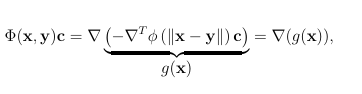
(4.2)
(xy)c is the gradient of a scalar function g. Note that the second argument of acts as a shift of the kernel and indicates where the eld (4.2) is centered. An interpolant to a curl-free vector eld u Rd sampled at distinct points X = xj N j=1 can be constructed from as follows:

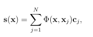
4.3

where the expansion coe cients cj Rd are found by enforcing the interpolation

condition s sX=uX .This result sin the linear system

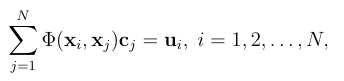
4.4

which is commonly written as Ac=u,where A is the block d N-by-d N interpolation matrix

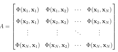
One can show that A is positive definite if is constructed from an appropriately chosen scalar-valued [22]; see Table 4.1for some examples. An important feature

Table 4.1 Examples of radial kernels that result in positive definite ma-trices A (4.5) for curl-free RBF interpolation. Here ε > 0 is the shape parameter.

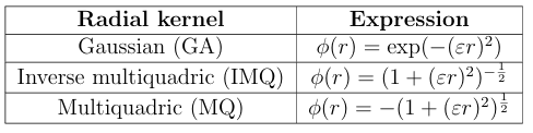
from the construction of the curl-free RBF interpolant is that we can extract a scalar potential for the interpolated eld by exploiting (4.2):

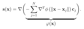
4.6

While the method described above will ensure a curl-free interpolant of the sam

pled eld, some issues do arise. First, the size of the linear system (4.4) grows rapidly with N, and, for a globally supported kernel, will be dense and computationally expensive to solve requiring O((dN)3) operations if a direct method is used. Second, each evaluation of the interpolant (or potential (4.6)) involves dN terms, which can become computationally expensive when many evaluations are necessary (such as occurs in the present application). Other issues involve the shape parameter used in the radial kernels from Table 4.1. This parameter controls how at or peaked the radial kernels are and has a dramatic e ect on both the accuracy of the interpolant as well as the conditioning of the interpolation matrix A. If is xed and the total number of interpolation points N grows, then the A matrix becomes exponentially ill-conditioned with N. Additionally, while extensive literature dedicated to nding the good values of to use exists for scalar RBF interpolation [10, 41], these approaches are computationally expensive, and this will only be exacerbated by the larger sizes of the linear systems for curl-free RBFs. To bypass these issues, we next discuss curl-free RBFs that do not feature a shape parameter. We address the issues with the computational cost in Section 4.3.

4.2.1 Curl-free polyharmonic splines

Polyharmonic spline (PHS) kernels were introduced by Duchon as a generalization of univariate splines to higher dimensions [19]. Scalar interpolants based on polyharmonic splines have the property that they minimize an energy functional that can be interpreted as a type of bending energy for the surface they produce, similar to univariate splines [55, ch. 13]. PHS are radial kernels and come in the following two types:

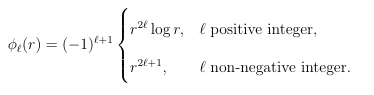
For interpolation in Rd, the rst option is typically used for d even and the second option for d odd. The choice for the order parameter is often made based on smoothness assumptions of the data, with larger for smoother data. However, larger also negatively e ects the numerical stability of the interpolants [55, ch. 12]. The combination of d and determines the minimization properties of the interpolants [55, ch. 13]; the choice of = 1 for d = 2 leads to the classical thin-plate spline. PHS do not feature a shape parameter like other RBFs, as any scaling of r just factors out of the kernels.

While is a free parameter, one does not need to continually search for a good value to use when the interpolation problem is changed, as is typically the case for RBFs with shape parameters. Curl-free PHS were introduced in [1] and have further been studied in [16, 4]. These matrix valued-kernels can be produced by using (4.1) with
given by either of the choices in (4.7) and chosen large enough to ensure the derivatives make sense; we denote these kernels by .

As with scalar PHS, it is necessary to modify the curl free RBF interpolant (4.3) to ensure a well-posed problem. In the curl-free PHS case, the interpolant (4.3) must be augmented with curl-free (vector) polynomials in Rd of
degree 1 [16], where degree refers to the total degree of any of the components of the (vector) polynomial. A basis for curl-free polynomials up to degree be generated as follows. Let p0 1 can pL be a monomial basis for scalar polynomials up to degree in Rd, where L = +d d 1 and p0 = 1. Then a basis for curl-free poly nomials up to degree 1, p1 pL , is given by applying the gradient to eachpi, i.e.pi= pi, i=1 L.A san example,we give the basis of degree 1and inR2andR3:

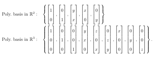
Acurl-free PHS interpolant of order to acurl-free vector field u Rd sampled
at distinct points X= xj N j=1 is givenas follows:

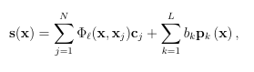
4.8

where the interpolation coefficient scj R d and bk R are determined by the condi tionssX
=uX as well as the constraints

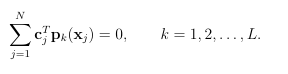
These constraints are necessary for the interpolant to minimize a certain energy norm and also limit its far- eld growth[16].We can state both constraints interms of the following linear system of equations:

[ A P] = [c] [u]
[ PT 0 ] = [ b] [0] ,

where A is defined in(4.5)and

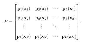
Provided the set of points X is uni solvent with respect to the curl-free polynomial basis(i.e.Pis fullrank),this linear system is non-singular and thus the interpolation problem is well-posed[16].However,as with in terpolation matrices based on curl-free RBF s with shape parameters, this interpolation matrix also becomes ill-conditioned
as N increases,but the growth is algebraic as opposed to exponential [22]. We note that a scalar potential can also be recovered similarly to(4.6)as

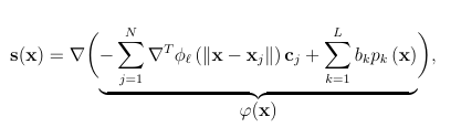
where pk are the scalar polynomial basis used to generate the curl-free poly nomial basis. This potential plays a key role in the CF P U method.

4.2.2 Example

At this point, it is illustrative to see how curl-free RBFs can be used to recover a level set from an oriented point cloud. We focus here on the case of a level curve in R2, since this is the situation in which the global method described above would be applicable due to the smaller problem sizes. The example we focus on uses the Cassini oval as the target level curve to recover, which can be described as the zero-level set of the implicit function

f(x) = f(x1 x2) = (x21 +x22)-2 2a2(x21 x22)+a4 -b4

where we take a = 1 and b = 11; seethe Figure 4.1(b) for the resulting curve (dashed line). We sample this curve at N nodes X = xj Nj=1 and compute the corresponding (unit) normal vectors using nj = f(xj); see Figure 4.1(a) for a plot of the exact data used for the case of N = 30. As mentioned in the introduction, the key to our method

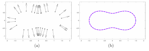
Figure 4.1 (a) N = 30 points sampled from a Cassini oval (4.11) with a = 1 and b = 11, together with the corresponding normal vectors to the curve. (b) The reconstruction from the global curl-free PHS interpolation method (magenta) with the exact curve (blue dashed line).

is the fact that the normal vectors to a level curve (or surface) are curl-free. We thus t the data (xj nj), j = 1
N, using the curl-free RBF interpolant (4.8) and from this extract out the potential as in (4.10). Since the potential for a curl-free eld is only unique up to a constant (which is a consequence of the Helmholtz decomposition theorem [8]), the zero-level curve of will not necessarily approximate the zero-level curve of f. To x this we set (x) = (x) , where is the discrete mean of at the nodes X. The result from this experiment is shown in Figure 4.1(b), where we see excellent agreement between the zero-level curve of and f. While this global method is reasonable to use for reconstring level curves (and surfaces) when N is small, the cost of solving the linear system (4.9) becomes too expensive for large N, which will be the case for any complicated surface from a sampled point cloud. We address this issue next.

4.3 CFPU method

Partition of unity (PU) methods o er a way to split up a global approximation prob lem on a domain intolocal approximation problems on overlapping patches covering. These local approximations are then blended together to form a global approximant using weight functions that form a partition of unity [2]. This procedure can drastically reduce the computational cost of the original approximation problem. In order to explain the CFPU method, we rst give a brief description of the idea behind PU methods as it pertains to our problem and introduce some necessary notation for what follows.

4.3.1 PU methods

Letf : Rd be an open, bounded domain of interest for approximating some function
R. Let 1M be a collection of distinct overlapping patches that form an open cover of , i.e., M
m=1 m , and let the overlap between patches be limited such that at most K << M patches overlap at any given point x . For each m=1 M, letwm: m [01]beaweightfunction such that wm is compactly supported on m, and let the set of weight functions wm have the property that M m=1 wm 1. Suppose sm is some approximation to f on each patch m. Then the PU approach of Babuska and Melenk [2] is to form an approximant s to f over the whole domain by blending the local approximants sm with wm as follows: s = M m=1 wmsm. Common choices for patches are disks for problems in R2 and balls for problems in R3. Based on these choices, weight functions wm can be easily constructed using Shepards method [46] as follows. Let : R+ R have compact support over the interval [01). For each patch m, let m denote its center and m > 0 denote its
radius, and de ne m(x) := ( x m m). The weight function for patch m is then given b

4.12

Note that each wm is only supported over m and that the summation in the denom inator only involves terms that are non-zero over patch m, which is bounded by K. In this study, we choose the patches as balls, and use the C1 quadratic B-spline

4.13

to de ne the weight functions.

RBFs are commonly used with the PU approach to reduce the computationa

cost. They have been used for approximating a function from scattered samples (e.g. [54, 13, 14]) and solving di erential equations (e.g. [42, 31, 45]). Recently the present authors presented a PU method for interpolation of divergence-free and curl free vector elds [18], which is what the current approach is based on.

4.3.2 Description of CFPU

For brevity, we describe the CFPU method for reconstructing a zero level surface P in R3 de ned by f(x) = 0 using curl-free PHS of order . Let X = xj Nj=1 be a given set points on P and let nj N j=1 denote the unit normals (or approximations to the normals) of P at X. Let 1 M be a set of overlapping patches that form an open cover of P such that each patch contains at least nmin nodes from X. Finally, let Xm denote the nodes contained in m and nm denote the cardinality of Xm. For each m, we t a curl-free RBF interpolant sm of the form (4.8) to the normals at the points in Xm and then extract from this its scalar potential m using (4.10).

A natural rst approach to constructing a global potential for approximating the level surface P would be to blend these local potentials m using the PU weight functions wm into a PU approximant of the form = M m=1wm m. However, this will lead to an issue since each m is only unique up to a constant. This means that for two patches k and m that overlap, k and m may be shifted from one another in the overlap region, which would then lead to an inaccurate global PU approximant in the overlap. To x this issue we can shift each potential by a di erent constant so that they approximately agree in the overlap region. To determine these constants, we use the fact that the points Xm reside on the zero level surface P, and we want each potential m to be approximately zero on Xm. One way to achieve this result is to enforce that the discrete mean of the local potentials is zero over the patch nodes.

To this end, let m denote the the discrete mean of m, and then de ne the shifted potential

m := m m

The global CFPU approximant for the underlying implicit function f is then given by

(x) := sum of m=1wm(x) m(x) .

We can then approximate P as the surface de ned by the set of all x in Mm=1 m suchthat (x) = 0. The CFPU method requires solving M linear systems of size (3nm+L)-by-(3nm+L) rather than one large (3N + L)-by-(3N + L) system for the global CF method described in Section 4.2.2. We select nm << N, for all m so that this results in a
signi cant savings, i.e. O( Mm=1 (3nm+L)3N) rather than O((3N+L)3), when using a
direct solver.

Furthermore, each of these smaller systems can be solved independently, making the CFPU method pleasingly parallel compared to the global method. Finally we note that the computational complexity for evaluating the CFPU approximant (4.14) is also signi cantly less than the global method. For each evaluation point, only a small subset (equal to the number of patches that contain the evaluation point) of the local potentials m need to be evaluated. The cost of evaluating each m is O(3nm+L) rather than O(3N +L) for the global method. These potentials can also be evaluated independently.

4.3.3 Exact interpolation

The CFPU method as described above will not in general exactly interpolate the zero level surface P at the points in X, i.e. (xj)= 0, j = 1 N, which is often desirable when the points are assumed to be exactly on the surface [34]. We can, however, enforce this condition by simply subtracting an interpolant of the residual from each patch potential m. We describe the details of this procedure below. Let the points in patch m from X be denoted by Xm = xm j nm j=1 and let m be a scalar PHS interpolant to the values of m at Xm. Using the same notation from Section 4.2.1, this interpolant can be written as

4.15

where the coe cients are determined from the interpolation conditions mXm= m X mand the moment conditions nmj=1cm j pk(xm j ) = 0, k = 0 m on patch m can be shifted by m to obtain

m := m m

By construction, this shifted potential satis es m(xm j ) = 0, so that an interpolatory global CFPU approximant for the underlying implicit function f can then be obtained as

4.16

An approximation to the surface P is again given as the set of all x in M m=1 m such that (x) = 0. We note that this exact interpolation technique is more expensive than just shifting the potentials by the mean as in (4.14), but only by a constant factor. Additionally, just as with m, each m can be determined independently of the others. The residual of the patch potentials m can be highly oscillatory, which could lead to spurious oscillations in the interpolants m and hence also . For 3D reconstructions, we thus recommend using the PHS kernel 0 (i.e. 0(r) = r) for the residual since the function will have minimal bending energy among all interpolants [19]. This is the choice we use in all of our examples.

4.3.4 Regularization

Normals

If the samples of the normal vectors of P are corrupted with noise, then interpolating them exactly on each patch to recover the potentials may cause issues, such as pro ducing spurious sheets in the reconstructed surface. In this case, it may make sense to instead introduce some regularization in the vector approximants on the patches. Regularized kernel approximation, such as smoothing splines or ridge regression [51], o ers one e ective way to do this. For curl-free PHS vector approximant s given in (4.8), the smoothing spline reg ularization approach amounts to solving the following minimization problem:

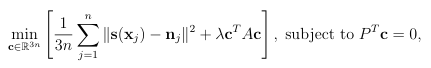
4.17

where A and P are the matrices from (4.9) for n points. The rst term in the quadratic functional measures the goodness of t of the approximant while the second term measures its smoothness.1 The regularization parameter
0 controls the tradeo between these terms, with larger resulting in smoother approximants. For a given , we can obtain the minimizer of the constrained quadratic functional (4.17) by solving the following modi ed version of the system (4.9):

[A+3n I P] [ c]=[ u]
[PT 0] [ b]=[0 ],

where I is the 3n-by-3n identity matrix and u contains the normals. In the CFPU method, we use this regularization approach on each patch m to obtain regularized potentials m. This opens up the option of using a different regularization parameter m on each patch, and thus controlling the regularization of the approximants spatially.

Residual

If the point samples in the point cloud are also noisy, as often occurs in range scans of real 3D objects, then enforcing exact interpolation on the patch potentials by interpolating the residual may again cause issues in the reconstruction. We can also introduce regularization in this process using smoothing splines. In this case, one uses a similar minimization problem as (4.17), but for the scalar TPS approximant (4.15). In fact, smoothing splines were developed for this type of problem [51]. Since different regularization parameters can be used for tting the normals vs. tting the residual of the potential, we let avoid confusion.

denote this parameter for the latter method to 1This term arises from the minimization of a Hilbert space semi-norm related to the function space of the vector approximants the so called native space norm associated with the kernel [4].

4.4 Additional algorithmic details

Here we describe some additional algorithmic aspects of the CFPU method not given above.

Unknown normals

While we have assumed the normals for the underlying level-set P are given, this may not always be the case for a given point cloud. Fortunately, however, there are many algorithms available that can approximate the normals directly from from the point cloud data Y ; see, for example, [53, 26, 39, 30].

Choosing the PU patches

One of the steps of CRBF-PU that can be an issue is the need to nd PU patch centers. For the results in section 4.5, we used Poisson disk sampling as implemented in Meshlab [15]. Depending on the size of the point cloud data, this step can be potentially prohibitive. Once the PU patch centers are found, the algorithm depends on kd-trees for range-queries in order to nd which sample points are on each patch. Again the number of data samples will be a determining factor in the speed of this step. The curl-free RBF linear system is then solved on each patch directly using LU decomposition. Since these systems are of size n << N, this is not as much of a computational concern.

Regularization parameter

Another step that one must consider with this algorithm is choosing the smoothing parameter, . While this can be chosen in an ad hoc fashion, it can also be automated using the GCV process [3].

Isosurface extraction

The last step of CFPU is to extract the isosurface from the computed potential approximant/interpolant. Currently the most popular algorithms for this are marching cubes [33] and dual-contouring [27]. The results presented in section 4.5 were created using the isosurface function in MATLAB (which uses marching cubes) on a su ciently dense grid.

4.5 Results

In this section we test the CFPU method on several di erent surface reconstructions. We start with a known surface to test the accuracy of the method. We then use the same problem, but we add noise to the normals in order to show how regularization can help reconstruct smooth surfaces to the data. We then consider a problem with raw range data that contains misalignments of the points and noise. Lastly we show how the method performs on various common surface reconstruction problems found in the literature. A goal of the tests is to show how the method parameters, such as the order for the curl-free PHS kernels a ect the reconstructions.

4.5.1 Accuracy of the method

We consider the surface generated from a (2,5) torus knot. The 3D curve de ning
the knot can be written parametrically as

(x(t) y(t) z(t)) = (cos(2t)(cos(5t) + 3) sin(2t)(cos(5t) + 3) sin(5t)),

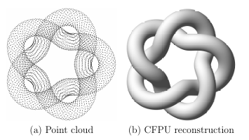
Figure 4.2 (a) N = 6144 point cloud and corresponding normals for the knot. (b) CFPU reconstruction of the knot from the data in part (a).

where 0 t 2 . We de ne the surface as a tube of radius 07 enclosing the curve, where the center of any circular cross section of the tube contains a point on the curve as its center. We generated N points X = x1 xN on this surface and the corresponding (unit) normals from the parametric representation. Figure 4.2(a) shows an example point set for N = 6144, while Figure 4.2(b) shows the reconstruction of the knot using the CFPU method with M = 864 patches and the exact interpolation method.

To test the accuracy of the CFPU method for approximating a potential for this surface, we sample the potentials at a set of 131424 points exactly on the knot and computed the di erence between these values and the exact solution. Since these evaluation points are on the surface, which we take to be the zero-level set of the knot, the exact solution should be zero. Table 4.2 displays the root mean square (RMS) and max-norm errors for the reconstructed potentials as the number of samples N grows. The table contains results for the potentials constructed using the curl-free PHS kernel for = 1 2, to show how the smoothness of the kernel a ects the accuracy. The sampling is chosen so that the average spacing between points decreases like N 12.
We see from the table that for both =1 and =2, the CFP U method appears to be converging to true zero-level surface as the density of the samples increases. Further more,we see that the overall errors are smaller when using the =2, and the convergence rate is higher. This is expected since the surface is smooth.

Table 4.2 Comparison of the errors in the CFPU reconstruction of the knot for increasing numbers of samples N using the curl-free PHS kernel ΦŜ, for Ŝ = 1, 2. All results use a fixed number of M = 864 PU patches and a fixed patch radius of δ = 3/4.

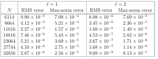
4.5.2 Reconstructions of a noisy surface

In this test, we demonstrate how the regularization procedures from Section 4.3.4 can help with noisy normals. We use the knot example from the previous section and add noise to the exact normals n1 nN according to

nj = nj + j

where j R3 and each component is a normally distributed random variable with mean zero and standard deviation 0.3. The rst column of Figure 4.3 shows the results for both theme an shift and

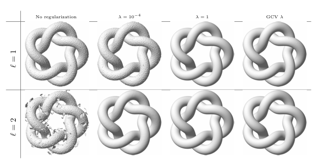
Figure 4.3 Comparison of the CFPU reconstructions of the knot with zero mean Gaussian white noise added to the normals. First column shows the reconstructions without any regularization. Second and third columns show the reconstructions using regularization with a xed parameter chosen for all the patches. Fourth column shows the reconstructions with the regularization parameter chosen using GCV on each patch. All results use N = 23064 samples and M = 864 patches with a xed patch radius of = 34.

exact interpolation versions of CFPU with no regularization. We can see from these gures that both methods result in very rough surfaces with spurious sheets. The next three columns of the gure show the reconstructions of both methods using the two regularization procedures from Section 4.3.4. The results in the second column use smoothing splines with a xed regularization parameter of = 10 2, while the third column uses GCV to select the regularization parameter on a per-patch basis.

The fourth column shows the results using regression splines where the number of centers for patch j is chosen as nj c = min(max(nj 6 18) n). We see that all the regularization techniques signi cantly reduce the noise in the reconstructions, but that the ones based on smoothing splines with the exact interpolation method give

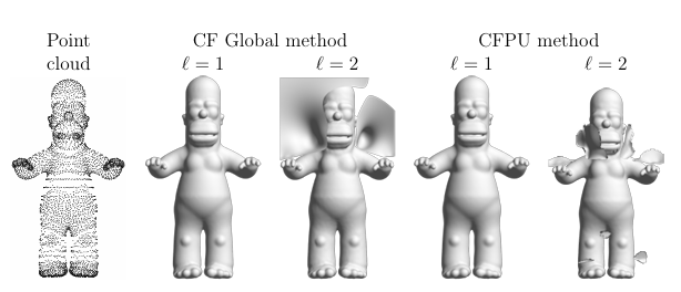
Figure 4.4 CFPU reconstructions of the Stanford bunny with (a) no regu-larization and (b) with regularization. In (b) GCV was used to determine the regularization parameter on each patch. Both experiments used the highest resolution zippered model of the bunny consisting of N = 35947 points and normals vectors and M = 848 patches.

the best results.

4.5.3 Standard test surfaces

We now focus on standard test problems from the literature, namely the Stanford Bunny, (2) Happy Buddha, (3) Dragon, (4) and Armadillo. The points for these models were obtained from high resolution triangulated surfaces of these objects provided by the Stanford University Computer Graphics Laboratory. Normal vectors for the surfaces were obtained from the MeshLab software package [15] after importing these triangulated surfaces. We generate surfaces from these points and normals using the CFPU method both with and without regularization. For the latter method, we use GCV to determine the regularization parameters. The results for the Stanford Bunny are shown in Figure 4.5. We see that without regularization (part (a)) the reconstruction is good, but that there are some spurious zero-level surfaces that result from the reconstructed potentials to the data around

Figure 4.5 CFPU reconstructions of the Stanford bunny with (a) no regu-larization and (b) with regularization. In (b) GCV was used to determine the regularization parameter on each patch. Both experiments used the highest resolution zippered model of the bunny consisting of N = 35947 points and normals vectors and M = 848 patches.

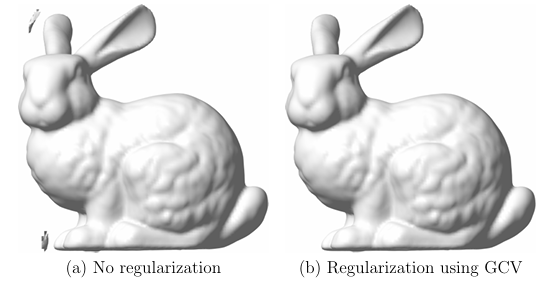
the ears and feet of the bunny. However, with regularization (part (b)) these spurious surfaces are removed without a reduction or smoothing of the details of the bunny. Figure 4.6 shows the surface reconstructions for the Dragon. The standard method again provides a good surface reconstruction in all but a few areas where some spurious zero-level surfaces appear. Including regularization removes these spurious surfaces, again without any noticeable over-smoothing. The reconstructions of the Armadillo are shown in Figure 4.7. We see from the gure that the standard method again gives a good reconstruction of the surface, but has a couple of spurious zero-level sets near the ngers and ears of the Armadillo. With regularization these are removed, and the resulting surface does not show any over-smoothing e ects. Finally, the results for the Happy Buddha are shown in Figure 4.8. From this

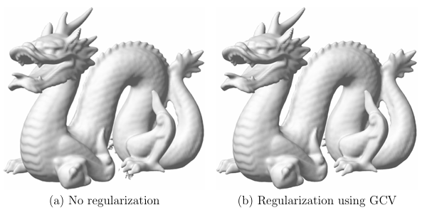
Figure 4.6 CFPU reconstructions of the Dragon with (a) no regularization and (b) with regularization. In (b) GCV was used to determine the regularization parameter on each patch. Both experiments used the high est resolution zippered model of the dragon consisting of N = 436418 points and normals vectors and M = 14400 patches.

figure we see that the reconstructed surface without regularization has some issues with spurious oscillations around the bottom of Happy Buddhas robe as well as the bottom of the base of the stand. Regularization with GCV does eliminate some of the issues, without over smoothing, but not all of them, especially for the bottom of the base. This a di cult area to construct an implicit surface too since the actual scanned object has a hole here.

4.6 Concluding remarks

In this work, we introduced the CFPU method, a novel method for implicit surface reconstruction based on a curl-free radial basis function partition of unity. We discussed a regularization for noisy data as well as a modi cation for exact surface interpolation. For future work, we will automate choosing the patches from the point

Figure 4.7 CFPU reconstructions of the Armadillo with (a) no regularization and (b) with regularization. In (b) GCV was used to determine the regularization parameter on each patch. Both experiments used the highest resolution zippered model of the dragon consisting of N = 172974 points and normals vectors and M = 14349 patches

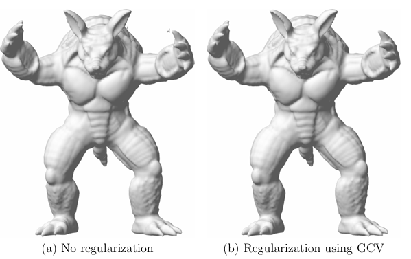
clouds and adapt the size and shape of the patches to better conform to the surface. We will also implement a least squares regularization and a parallelization of the algorithm for even further improvements on computational e ciency.

Acknowledgements

KPDs work was partially supported by a SMART Scholarship, which is funded by The Under Secretary of Defense-Research and Engineering, National Defense Education Program / BA-1, Basic Research. GBWs work was partially supported by National Science Foundation grant CCF 1717556. The Stanford Bunny, Happy Buddha, Dragon, and Armadillo data were obtained from the Stanford University Computer Graphics Laboratory.

Figure 4.8 CFPU reconstructions of the Happy Buddha with (a) no
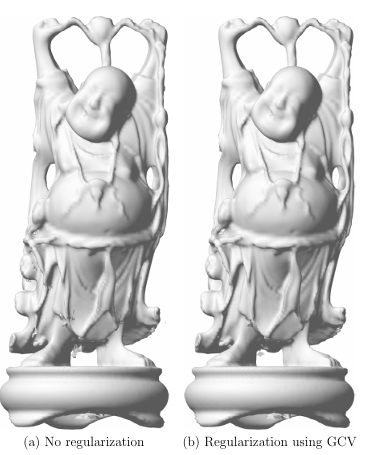
regu-larization and (b) with regularization. In (b) GCV was used to
determine the regularization parameter on each patch. Both experiments used the highest resolution zippered model of the dragon consisting of N = 583079 points and normals vectors and M = 14226 patches.

REFERENCES

[1] L. Amodei and M. N. Benbourhim. A vector spline approximation. J. Approx. Theory, 67(1):5179, 1991.

[2] I. Babuska and J. M. Melenk. The partition of unity method. Int. J. Numer. Meths. Eng., 40:727758, 1997.

[3] D. M. Bates, M. J. Lindstrom, G. Wahba, and B. S. Yandell. Gcvpack- routines for generalized cross validation. Communications in Statistics- Simulation and Computation, 16(1):263297, 1987.

[4] M. N. Benbourhim and A. Bouhamidi. Meshless pseudo-polyharmonic divergence-free and curl-free vector elds approximation. SIAM J. Math. Anal., 42(3):12181245, 2010.

[5] M. Berger, J. Levine, L. Nonato, G. Taubin, and S. C.T. A benchmark for surface reconstruction. ACM Trans Graph, 32(2):20:120:17, 2013.

[6] M. Berger, A. Tagliasacchi, L. M. Seversky, P. Alliez, G. Guennebaud, J. A. Levine, A. Sharf, and C. T. Silva. A survey of surface reconstruction from point clouds. Comput. Graph. Forum, 36(1):301329, 2017.

[7] M. Berger, A. Tagliasacchi, L. M. Seversky, P. Alliez, J. A. Levine, A. Sharf, and C. T. Silva. State of the art in surface reconstruction from point clouds. In Eurographics 2014- State of the Art Reports, 2014.

[8] H. Bhatia, G. Norgard, V. Pascucci, and P.-T. Bremer. The Helmholtz-Hodge decomposition a survey. IEEE Transactions on Visualization and Computer Graphics, 19(8):13861404, 2013.

[9] F. Calakli and G. Taubin. SSD: Smooth signed distance surface reconstruction. Comput Graph Forum, 30(7):493501, 2011.

[10] R. E. Carlson and T. A. Foley. The parameter r2 in multiquadric interpolation. Comput. Math. Appl., 21:2942, 1991.

[11] J. C. Carr, R. K. Beatson, J. B. Cherrie, T. J. Mitchell, W. R. Fright, B. C. McCallum, and T. R. Evans. Reconstruction and representation of 3d objects with radial basis functions. In Proceedings of the 28th Annual Conference on Computer Graphics and Interactive Techniques, pages 6776, 2001.

[12] J. C. Carr, W. R. Fright, and R. K. Beatson. Surface interpolation with radial basis functions for medical imaging. IEEE Transactions on Medical Imaging, 16(1):96107, 1997.

[13] R. Cavoretto and A. De Rossi. Fast and accurate interpolation of large scattered data sets on the sphere. Comput. Appl. Math., pages 15051521, 2010. [14] R. Cavoretto, A. De Rossi, and E. Perracchione. Partition of unity inter polation on multivariate convex domains. Int. J. Model. Simul. Sci. Comp., 06(04):1550034, 2015.

[15] M. Corsini, P. Cignoni, and R. Scopigno. E cient and exible sampling with blue noise properties of triangular meshes. IEEE Transaction on Visualization and Computer Graphics, 18(6):914924, 2012.

[16] F. Dodu and C. Rabut. Vectorial interpolation using radial-basis-like functions. Comput. Math. Appl., 43(3-5):393411, 2002. Radial basis functions and partial differential equations.

[17] F. Dodu and C. Rabut. Irrotational or divergence-free interpolation. Numer. Math., 98(3):477498, 2004.

[18] K. P. Drake, E. J. Fuselier, and G. B. Wright. A divergence-free and curl-free radial basis function partition of unity method. arXiv:2010.15898, 2020.

[19] J. Duchon. Splines mimimizing rotation-invariant semi-norms in Sobolev space. Constr. Theory Funct. of Several Variables, Springer Lecture Notes in Math, 21:85100, 1977.

[20] G. E. Fasshauer. Meshfree Approximation Methods with MATLAB, Interdisciplinary Mathematical Sciences. World Scienti c Publishers, Singapore, 2007.

[21] B. Fornberg and N. Flyer. A Primer on Radial Basis Functions with Applications to the Geosciences. SIAM, Philadelphia, 2014.

[22] E. J. Fuselier. Sobolev-type approximation rates for divergence-free and curl-free RBF interpolants. Math. Comput., 77(263):14071423, 2008.

[23] E. J. Fuselier and G. B. Wright. A radial basis function method for computing Helmholtz-Hodge decompositions. IMA J. Numer. Anal., 37(2):774797, 2017.

[24] J. Gois, V. Polizelli-Junior, T. Etiene, E. Tejada, A. Castelo, L. Nonato, and T. Ertl. Twofold adaptive partition of unity implicits. Vis Comput, 24(12):1013 1023, 2008.

[25] H. Hoppe, T. DeRose, T. Duchamp, J. McDonald, and W. Stuetzle. Surface reconstruction from unorganized points. SIGGRAPH Comput. Graph., 26(2):71 78, 1992.

[26] S. Jin, R. R. Lewis, and D. West. A comparison of algorithms for vertex normal computation. The Visual Computer, 21:7182, 2005.

[27] T. Ju, F. Losasso, S. Schaefer, and J. Warren. Dual contouring of hermite data. ACM Trans. Graph., 21(3):339346, 2002.

[28] M. Kazhdan, M. Bolitho, and H. Hoppe. Poisson surface reconstruction. In Proceedings of symposium on geometry processing, pages 6170, 2006.

[29] M. Kazhdan and H. Hoppe. Screened poisson surface reconstruction. ACM Trans Graph, 32(3):29, 2013.

[30] K. Klasing, D. Altho , D. Wollherr, and M. Buss. Comparison of surface normal estimation methods for range sensing applications. In IEEE International Conference on Robotics and Automation, pages 32063211, 2009.

[31] E. Larsson, V. Shcherbakov, and A. Heryudono. A least squares radial basis function partition of unity method for solving PDEs. SIAM J. Sci. Comput., 39(6):A2538A2563, 2017.

[32] S. Liu, C. C. Wang, G. Brunnett, and J. Wang. A closed-form formulation of HRBF-based surface reconstruction by approximate solution. Comput. Aided Des., 78(C):147157, 2016.

[33] W. E. Lorensen and H. E. Cline. Marching cubes: A high resolution 3D surface construction algorithm. SIGGRAPH Comput. Graph., 21(4):163169, 1987.

[34] I. Macedo, J. P. Gois, and L. Velho. Hermite radial basis functions implicits. Computer Graphics Forum, 30(1):2742, 2011.

[35] B. S. Morse, T. S. Yoo, P. Rheingans, D. T. Chen, and K. R. Subramanian. Interpolating implicit surfaces from scattered surface data using compactly sup ported radial basis functions. In Proceedings International Conference on Shape Modeling and Applications, pages 8998, 2001.

[36] Y. Ohtake, A. Belyaev, M. Alexa, G. Turk, and H. P. Seidel. Multi-level partition of unity implicits. ACM Trans. Graph., 22(3):463470, 2003.

[37] Y. Ohtake, A. Belyaev, and H. P. Seidel. 3D scattered data interpolation and approximation with multilevel compactly supported RBFs. Graph Models, 67:150 165, 2005.

[38] Y. Ohtake, A. Belyaev, and H. P. Seidel. Sparse surface reconstruction with adaptive partition of unity and radial basis functions. Graph Models, 68(1):15 24, 2006.

[39] D. OuYang and H.-Y. Feng. On the normal vector estimation for point cloud data from smooth surfaces. Computer-Aided Design, 37(10):10711079, 2005.

[40] R. Pan, X. Meng, and T. Whangbo. Hermite variational implicit surface recon struction. Sci China Ser F, 52(2):308315, 2009.

[41] S. Rippa. An algorithm for selecting a good value for the parameter c in radial basis function interpolation. Adv. Comp. Math., 11:193210, 1999.

[42] A. Safdari-Vaighani, A. Heryudono, and E. Larsson. A radial basis function partition of unity collocation method for convectiondi usion equations arising in nancial applications. J. Sci. Comput., 64(2):341367, 2015.

[43] M. Samozino, M. Alexa, P. Alliez, and M. Yvinec. Reconstruction with voronoi centered radial basis functions. In Proceedings of the fourth Eurographics sym posium on geometry processing, pages 5160, 2006.

[44] V. Savchenko, A. Pasko, O. G. Okunev, and T. L. Kunii. Function representation of solids reconstructed from scattered surface points and contours. Comput Graph Forum, 14(4):181188, 1995.

[45] V. Shankar and G. B. Wright. Mesh-free semi-Lagrangian methods for transport on a sphere using radial basis functions. J. Comput. Phys., 366:170190, Aug. 2018.

[46] D. Shepard. A two-dimensional interpolation function for irregularly-spaced data. In Proceedings of the 1968 23rd ACM national conference, pages 517524, New York, NY, 1968. ACM Press.

[47] J. Sussmuth, Q. Meyer, and G. Greiner. Surface reconstruction based on hier archical oating radial basis functions. Comput Graph Forum, 29(6):18541864, 2010.

[48] I. Tobor, P. Reuter, and C. Schlick. Reconstructing multi-scale variational partition of unity implicit surfaces with attributes. Graph Models, 68(1):2541, 2006.

[49] G. Turk and J. F. OBrien. Shape transformation using variational implicit functions. In Proceedings of the 26th Annual Conference on Computer Graphics and Interactive Techniques, SIGGRAPH 99, pages 335342, 1999.

[50] G. Turk and J. F. OBrien. Modeling with implicit surfaces that interpolate. ACM Trans Graph, 21(4):855873, 2002.

[51] G. Wahba. Spline models for observational data. CBMS-NSF Regional Confer ence series in applied mathematics 59. Society for Industrial and Applied Mathematics, 1990.

[52] C. Walder, B. Scholkopf, and O. Chapelle. Implicit surface modeling with a globally regularised basis of compact support. Comput Graph Forum, 25(3):635 644, 2006.

[53] C. Wang, H. Tanahashi, H. Hirayu, Y. Niwa, and K. Yamamoto. Comparison of local plane tting methods for range data. volume 1, pages 663669, 02 2001.

[54] H. Wendland. Fast evaluation of radial basis functions : Methods based on partition of unity. In Approximation Theory X: Wavelets, Splines, and Applications, pages 473483. Vanderbilt University Press, 2002.

[55] H. Wendland. Scattered Data Approximation, volume 17 of Cambridge Monogr. Appl. Comput. Math. Cambridge University Press, Cambridge, 2005.

CHAPTER 5:
CONCLUSION

This dissertation introduced a collection of fast and accurate algorithms for analysis of data collected on irregular domains. In Chapter 2, we presented our rst paper in which we developed a method for calculating the angular power spectrum of the cosmic microwave background (CMB) radiation. We used numerical tests to demon strate our algorithms bene ts over the leading method in the HEALPix software for calculating the angular power spectrum of deterministic functions on the sphere. Future directions for this work include implementing the method in a low-level computing language, like C++, in order to improve run-time performance. Additionally, the method could be extended to include functionality for calculating the angular power spectrum for the polarization of CMB temperature maps.

In Chapter 3, the second paper presents the rst method for approximating divergence-free and curl-free vector elds in R2 and S2 and curl-free elds in R3 with a vector-valued radial basis function partition of unity method. We proved error-estimates for the approximants and demonstrated the high-order convergence rates of our method with numerical tests. An area of future work for this method is to work toward adapting it to be stable for RBFs in the at limit of the shape parameter . Additionally, extending the method to use a least squares approach for local interpolation on local PU patches could be useful for further reducing the computational cost and introducing some regularization for noisy data.

Finally our third paper is given in Chapter 4, in which we applied the technique of the second paper to the problem of implicit surface reconstruction from oriented point clouds. Our novel approach, titled CFPU, uses a curl-free RBF interpolation of the normal vectors to extract a potential for the reconstructed vector eld whose zero-level surface approximates the point cloud. We discussed a regularization for noisy data as well as a modi cation for exact surface interpolation. We then demon strated the e ectiveness of this method by reconstructing known surfaces as well as surfaces from scanned point clouds. Future work from the ideas developed in this paper could include investigating a computationally cheaper regularization approach based on least squares and an automated method for choosing the PU patches. Finally, parallelizing the algorithm would be important for further improvements on computational cost.

Trendigt

Terrormisstänkta prins Reuss advokat till DN: ”Min klient ville aldrig utöva våld”

Ett ödesval för klimatet och miljön – här är forskarnas viktigaste frågor

DN Debatt. ”Rimligt att Sverige sa nej till euron då – men inte nu”

Ståhl trea i Marrakech – långt efter vinnaren

Då ska du undvika löpning i värmen

Dissertation Example-A COLLECTION OF FAST ALGORITHMS FOR SCALAR AND VECTOR-VALUED DATA ON IRREGULAR DOMAINS: SPHERICAL HARMONIC ANALYSIS, DIVERGENCE-FREE/CURL-FREE RADIAL BASIS FUNCTIONS, AND IMPLICIT SURFACE RECONSTRUCTION by Kathryn Primrose Drake

A COLLECTION OF FAST ALGORITHMS FOR SCALAR AND VECTOR-VALUED DATA ON IRREGULAR DOMAINS: SPHERICAL HARMONIC ANALYSIS, DIVERGENCE-FREE/CURL-FREE RADIAL BASIS FUNCTIONS, AND IMPLICIT SURFACE RECONSTRUCTION

BOISE STATE UNIVERSITY GRADUATE COLLEGE

DEFENSE COMMITTEE AND FINAL READING APPROVALS

of the dissertation submitted by

Kathryn Primrose Drake

DEDICATION

ACKNOWLEDGMENTS

ABSTRACT

TABLEOFCONTENTS

LIST OF FIGURES

LIST OF TABLES

CHAPTER 1: INTRODUCTION

1.1 Cosmic Microwave Background Radiation Angular Power Spectrum

1.1.1 Motivation

1.1.2 Background

1.2 Scalar Radial Basis Function Interpolation

1.2.1 Motivation

1.2.2 Background

Table 1.1 Commonly used radial kernels, where the rst three are positive de nite, r = x y , and is the shape parameter.

1.3 Implicit Surface Reconstruction from Oriented Point Clouds

1.3.1 Motivation

1.4 Overview of the Dissertation

REFERENCES

CHAPTER 2:

A FAST AND ACCURATE ALGORITHM FOR SPHERICAL HARMONIC ANALYSIS ON HEALPIX GRIDS WITH APPLICATIONS TO THE COSMIC MICROWAVE BACKGROUND RADIATION

Abstract

2.1 Introduction

2.2 Background and Current Approach

2.2.1 HEALPix Scheme

2.2.2 HEALPix Software Spherical Harmonic Analysis

Pixel Weights and Ring Weights

2.3 HP2SPH

2.3.1 Step1: Transform the data to a tensor product latitude longitude grid

2.3.2 Step 2: Compute Bivariate Fourier Coe cients

Double Fourier Sphere (DFS) Method

Nonuniform Fast Fourier Transform (NUFFT)

2.3.3 Step 3: Obtain the spherical harmonic coefficients via the fast spherical harmonic transform (FSHT)

2.4 Numerical Results

2.4.1 Convergence of Spherical Harmonic Coefficients

2.4.2 Errors in the Angular Power Spectrum

2.4.3 Application to Real CMB Map

2.5 Conclusions and Remarks

Acknowledgements

Appendix A: Spherical Harmonic Conventions

REFERENCES

CHAPTER 3:

A DIVERGENCE-FREE AND CURL-FREE RADIAL BASIS FUNCTION PARTITION OF UNITY METHOD

Abstract

3.1 Introduction

3.2 Div/Curl-free RBFs

3.2.1 Notation and preliminaries

3.2.2 Div-free RBF interpolation

3.2.3 Curl-free RBF interpolation

3.3 A div-free/curl-free partition of unity method

3.3.1 Partition of unity methods

3.3.2 Description of the method

3.3.3 Implementation details

Patch centers

3.4 Error Estimates

Proposition.

3.5 Numerical experiments

3.5.1 Div-free eld on R2

3.5.2 Div-free eldonS2

3.5.3 Curl-free eld on the unit ball

3.6 Concluding remarks

Acknowledgments

REFERENCES

CHAPTER 4:

IMPLICIT SURFACE RECONSTRUCTION WITH A CURL-FREE RADIAL BASIS FUNCTION PARTITION OF UNITY METHOD

Abstract

4.1 Introduction

4.1.1 Relationship to previous work

4.1.2 Contributions

CHAPTER 1:
INTRODUCTION

1.1 Cosmic Microwave Background Radiation
Angular Power Spectrum

A DIVERGENCE-FREE AND CURL-FREE RADIAL BASIS FUNCTION PARTITION OF
UNITY METHOD

IMPLICIT SURFACE RECONSTRUCTION
WITH A CURL-FREE RADIAL BASIS
FUNCTION PARTITION OF UNITY METHOD

CHAPTER 5:
CONCLUSION